Ensemble Learning in Machine Learning: Methods, Techniques and Python Implementation

Quick Overview:

• Ensemble learning combines multiple machine learning models to produce stronger, more reliable predictions than relying on a single model.

• The four main methods are bagging, boosting, stacking, and voting, with each method combining models in a different way.

• Popular algorithms include Random Forest, AdaBoost, Gradient Boosting, XGBoost, Voting Classifier, and Stacking.

• In this blog you will explore ensemble learning in detail along with its techniques, Python implementation, advantages, disadvantages, popular algorithms and methods.

Build future-ready AI expertise with the Executive Post Graduate Certificate in Applied AI & Machine Learning. Develop practical skills in AI and machine learning to solve real-world problems and advance your career.

What Is Ensemble Learning in Machine Learning?

Ensemble learning in machine learning is built on a simple and powerful idea which combines predictions of several models, often called base learners, to produce better predictions rather than relying on any single model.

Rather than spending all of your effort trying to build one perfect model, ensemble technique in machine learning accepts that individual models will each have their own weaknesses and focuses on combining them so those weaknesses cancel out. 

Let’s understand what is ensemble learning in machine learning​ using an analogy below:

• Imagine you need to make an important decision, but you are not sure what the right answer is. Instead of asking just one person, you ask several people for their opinions.

• Each person may have different knowledge and may make different mistakes. But when you combine their answers, the final decision is often more reliable than relying on just one person.

This ensemble technique in machine learning is widely used in classification and regression problems and makes the foundation of methods such as Random Forest, AdaBoost, Gradient Boosting, and XGBoost. 

Ensemble learning gained global popularity during the 2009 Netflix Prize Competition, where the winning team ("BellKor’s Pragmatic Chaos") combined 107 different predictive models to achieve the target 10% improvement in recommendation accuracy and to win a $1 million prize.

Now let’s understand how ensemble learning in machine learning works.

How Does Ensemble Learning Algorithm Work?

The basic idea behind ensemble learning in machine learning is to train multiple models and then combine their predictions.

The process involves these key steps:

1. Select base models: First, choose one or more machine learning models to form the ensemble.

2. Train the models: Then, train the models using the available training data.

3. Generate predictions: Each model produces its own prediction.

4. Combine predictions: Use a suitable ensemble technique in machine learning to combine the individual outputs.

5. Generate the final prediction: The combined result becomes the ensemble's prediction.

For example, in a classification problem, five models may predict:

Model 1: Class A
Model 2: Class B
Model 3: Class A
Model 4: Class A
Model 5: Class B

With majority voting, the final prediction would be Class A.  The exact process depends on the ensemble learning methods being used. 

Now after exploring the working of ensemble learning, let’s see what different ensemble learning methods​ are available and understand how each one combines multiple models to improve prediction accuracy.

Also Read: Machine Learning Algorithms: Working, Types and Examples

Main Ensemble Learning Methods

There are four main ensemble learning methods including bagging, boosting, stacking, and voting. Each method combines models differently and is required to meet different modelling requirements.

1. Bagging

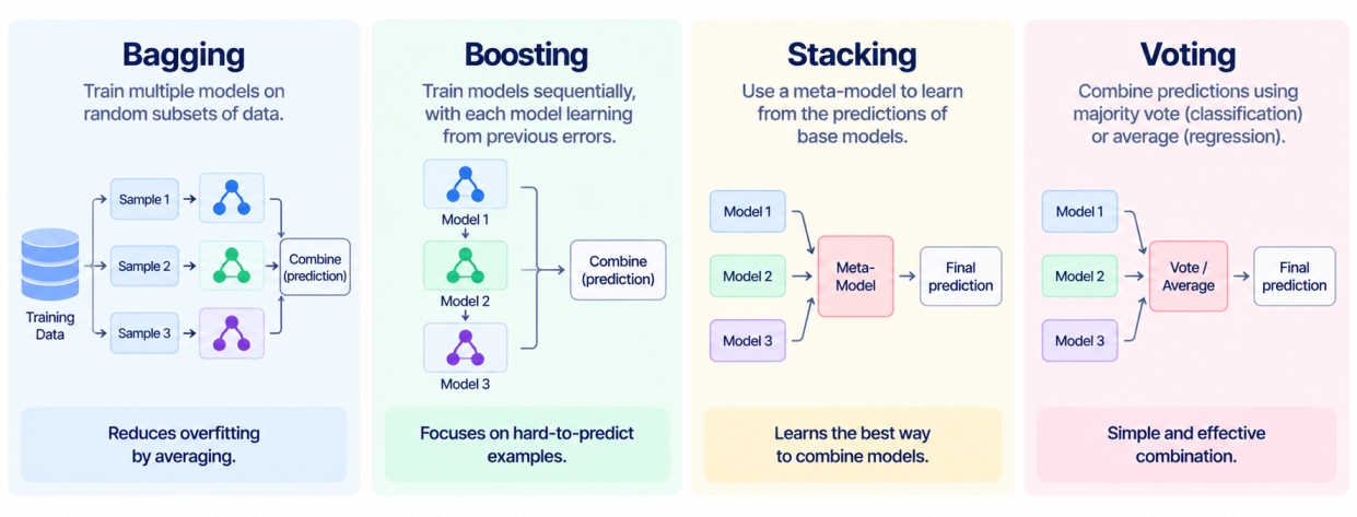
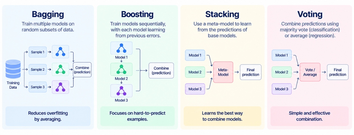
Bagging, short for bootstrap aggregating, trains multiple base models independently in parallel. Each model is trained on different random samples of the training data, then combines their predictions through voting for classification or averaging for regression.

How Does Bagging Work?

The process generally follows these key steps:

1. Create multiple bootstrap samples from the original dataset.

2. Train a separate model on each sample.

3. Generate predictions from all trained models.

4. Combine the predictions using averaging or voting.

Bootstrap Sampling

Bootstrap sampling creates different training datasets by randomly selecting data from the original dataset with replacement. This means the same data point can be selected more than once, while some data points may not be selected at all.

How Does Bagging Reduce Variance?

Bagging reduces the impact of individual model variations by combining predictions from multiple models. Since the models are trained on different samples, their errors may differ. Aggregating their predictions can make the final model more stable and reduce variance.

Example: Random Forest

Random Forest is a popular bagging-based ensemble technique in machine learning​ that combines multiple decision trees. Each tree contributes to the final prediction, helping create a more robust model than a single decision tree.

Also Read: Linear Regression in Machine Learning: Types, Algorithm, and Implementation

2. Boosting

Boosting is an ensemble technique in machine learning that builds models sequentially. Each new model focuses more on correcting errors made by previous models.

How Does Boosting Work?

The general process include these key steps:

1. Train an initial weak learner.

2. Identify errors made by the model.

3. Give greater attention to observations that were predicted incorrectly.

4. Train the next model to improve these predictions.

5. Repeat the process for multiple iterations.

Sequential Model Training

Unlike bagging, where models can be trained independently, boosting builds models one after another. Each new learner uses information from earlier learners to improve the overall ensemble.

How Does Boosting Focus on Errors?

Boosting gives additional importance to observations that previous models handled poorly. This allows subsequent models to concentrate on difficult cases and gradually improve the combined model.

Examples of Boosting

Popular boosting methods include:

• AdaBoost

• Gradient Boosting

• XGBoost

Also Read: K Means Clustering in Machine Learning: Algorithm, Steps, Examples, and Applications

3. Stacking

Stacking combines predictions from multiple different base models using another model called a meta-model.

How Does Stacking Work?

Suppose you use Logistic Regression, Decision Tree, and KNN as base learners. Each model produces predictions, and these predictions are passed to a meta-model. The meta-model learns how to combine the outputs and produces the final prediction.

1. Base Models

2. Predictions

3. Meta-Model

4. Final Prediction

When Is Stacking Useful?

Stacking can be useful when different models capture different patterns in the data. Combining their predictions allows the meta-model to learn which outputs are more useful for making the final prediction.

4. Voting

Voting combines predictions from multiple models to determine the final classification. There are three common approaches for voting:

Hard Voting

Hard voting selects the class that receives the most votes from the individual models.

For example:

• Model 1: Cat

• Model 2: Dog

• Model 3: Dog

• Model 4: Dog

• Model 5: Cat

The final prediction is Dog because it receives the majority of votes.

Also Read: Clustering in Machine Learning: Types, Algorithms, Examples, and How It Works

Soft Voting

Soft voting combines the predicted probabilities from different models and selects the class with the highest combined probability.

Example:
Suppose three models predict whether an email is Spam or Not Spam:

Average probability:

• Spam = 70%

• Not Spam = 30%

Final prediction: Spam, because it has the higher combined probability.

Also Read: Supervised vs Unsupervised Learning: Differences, Examples, and Applications

Weighted Voting

Weighted voting gives some models greater influence than others. A model considered more reliable can receive a higher weight when calculating the final prediction.

Example:
Suppose three models predict whether a customer will Buy or Not Buy. Model 1 is more accurate, so it gets a higher weight.

• Model 1: Buy- Weight 3

• Model 2: Not Buy- Weight 1

• Model 3: Not Buy- eight 1

Weighted votes:

• Buy = 3

• Not Buy = 2

Final prediction: Buy, because the more reliable Model 1 has a greater influence on the final result.

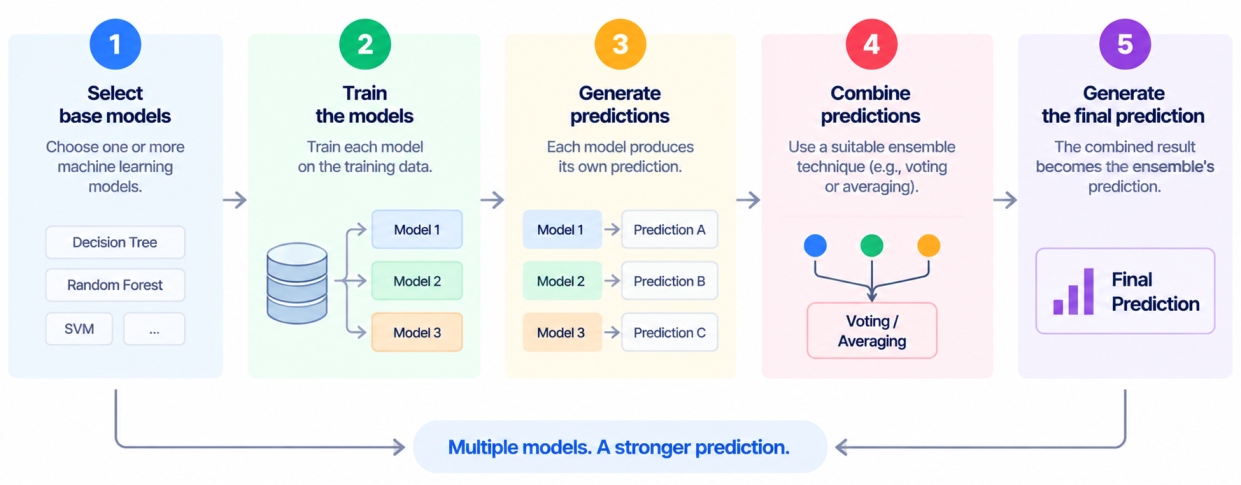
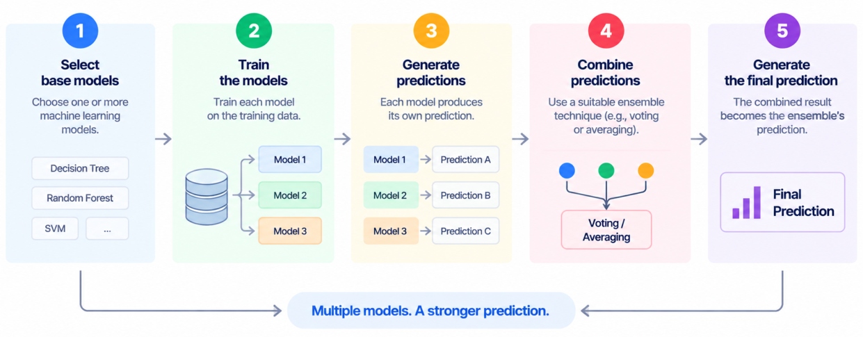
So, these are some majorly used ensemble learning methods​ used to train models. Now let’s explore what are some of the popular ensemble learning algorithms.

Popular Ensemble Learning Algorithms

There are several widely used ensemble learning algorithms which are built around the methods discussed above in methods.

Now let’s explore how to implement the ensemble learning techniques in machine learning using Python.

Also Read: Support Vector Machine (SVM) in Machine Learning: Algorithm, Types, Kernels, and Examples

How to Implement Ensemble Learning in Python

In this example, we will use Python and scikit-learn to build different ensemble learning models and compare their performance with individual base models. 

1. Import Required Libraries

• NumPy is used to create and work with numerical data.

• Pandas is used to create and manage the dataset.

• Scikit-learn provides the models, data splitting, scaling, and evaluation tools.

• Decision Tree, Logistic Regression, and KNN are used as base learners.

• Random Forest, AdaBoost, Gradient Boosting, Voting, and Stacking are used as ensemble models.

• Accuracy and F1-score are used to measure model performance.

import numpy as np

import pandas as pd

from sklearn.model_selection import train_test_split

from sklearn.preprocessing import StandardScaler

from sklearn.tree import DecisionTreeClassifier

from sklearn.linear_model import LogisticRegression

from sklearn.neighbors import KNeighborsClassifier

from sklearn.ensemble import (

    RandomForestClassifier, AdaBoostClassifier,

    GradientBoostingClassifier, VotingClassifier, StackingClassifier

)

from sklearn.metrics import accuracy_score, f1_score

2. Prepare the Dataset

• A sample dataset of 400 loan applications is created.

• Income, credit score, and existing loans are used as input features.

• A score is calculated using these features and some random noise.

• The score is used to determine whether a loan is approved or rejected.

• The data is divided into training and testing sets.

• The features are scaled before being given to the models.

np.random.seed(42)

n = 400

income = np.round(np.random.uniform(20000, 120000, n))

credit_score = np.round(np.random.uniform(300, 850, n))

existing_loans = np.random.randint(0, 4, n)

score = (income / 120000) 0.5 + (credit_score / 850) 0.5 - existing_loans * 0.1

approved = ((score + np.random.normal(0, 0.12, n)) > 0.45).astype(int)

df = pd.DataFrame({

    "Income": income,

    "CreditScore": credit_score,

    "ExistingLoans": existing_loans,

    "Approved": approved

})

X = df[["Income", "CreditScore", "ExistingLoans"]]

y = df["Approved"]

X_train, X_test, y_train, y_test = train_test_split(

    X, y, test_size=0.2, random_state=42, stratify=y

)

scaler = StandardScaler()

X_train_scaled = scaler.fit_transform(X_train)

X_test_scaled = scaler.transform(X_test)

This dataset of 400 loan applications includes a deliberately high level of noise, which makes it a more realistic test of whether ensembling actually helps, since ensembles provide the least benefit on data that is already trivially easy to classify.

3. Select Base Learners

• A Decision Tree is created with a maximum depth of 4.

• Logistic Regression is created as a linear model.

• KNN is created with 7 nearest neighbours.

• These models will be used individually and later as part of ensembles.

dt = DecisionTreeClassifier(max_depth=4, random_state=42)

lr = LogisticRegression(random_state=42)

knn = KNeighborsClassifier(n_neighbors=7)

These three base learners are chosen specifically because they work in fundamentally different ways, a rule-based tree, a linear probabilistic model, and a distance-based model, which is exactly the diversity that makes an ensemble worthwhile.

4. Train Individual Models

• Each base model is trained using the training data.

• Predictions are made on the test data.

• Accuracy and F1-score are calculated for each model.

• These scores give us a baseline for comparing the ensemble technique in machine learning​.

for name, model in [("Decision Tree", dt), ("Logistic Regression", lr), ("KNN", knn)]:

    model.fit(X_train_scaled, y_train)

    pred = model.predict(X_test_scaled)

    print(f"{name}: accuracy={accuracy_score(y_test, pred):.4f}, f1={f1_score(y_test, pred):.4f}")

5. Combine Model Predictions

• Hard Voting combines the class predictions from all three models.

• Soft Voting combines their predicted probabilities.

• Stacking combines predictions from multiple models and passes them to a Logistic Regression meta-model.

• The ensemble models are then trained on the training data.

vote_hard = VotingClassifier(

    estimators=[("dt", dt), ("lr", lr), ("knn", knn)], voting="hard"

)

vote_hard.fit(X_train_scaled, y_train)

vote_soft = VotingClassifier(

    estimators=[("dt", dt), ("lr", lr), ("knn", knn)], voting="soft"

)

vote_soft.fit(X_train_scaled, y_train)

stack = StackingClassifier(

    estimators=[

        ("dt", DecisionTreeClassifier(max_depth=4, random_state=42)),

        ("knn", KNeighborsClassifier(n_neighbors=7)),

        ("rf", RandomForestClassifier(n_estimators=100, max_depth=6, random_state=42))

    ],

    final_estimator=LogisticRegression(),

    cv=5

)

stack.fit(X_train_scaled, y_train)

6. Evaluate the Ensemble

• Random Forest, AdaBoost, and Gradient Boosting models are created.

• All ensemble learning methods are trained on the training data.

• Each model predicts the loan approval results.

• Accuracy and F1-score are calculated for every ensemble.

rf = RandomForestClassifier(n_estimators=200, max_depth=6, random_state=42)

ada = AdaBoostClassifier(n_estimators=100, random_state=42)

gb = GradientBoostingClassifier(n_estimators=150, learning_rate=0.1, max_depth=3, random_state=42)

models = [

    ("Voting (hard)", vote_hard), ("Voting (soft)", vote_soft),

    ("Stacking", stack), ("Random Forest", rf),

    ("AdaBoost", ada), ("Gradient Boosting", gb)

]

for name, model in models:

    if name not in ("Voting (hard)", "Voting (soft)", "Stacking"):

        model.fit(X_train_scaled, y_train)

    pred = model.predict(X_test_scaled)

    print(f"{name}: accuracy={accuracy_score(y_test, pred):.4f}, f1={f1_score(y_test, pred):.4f}")

Output:

Decision Tree: accuracy=0.7250, f1=0.7440

Logistic Regression: accuracy=0.7750, f1=0.7960

KNN: accuracy=0.7750, f1=0.7910

Voting (hard): accuracy=0.7880, f1=0.8050

Voting (soft): accuracy=0.8000, f1=0.8180

Stacking: accuracy=0.7880, f1=0.8050

Random Forest: accuracy=0.7630, f1=0.7820

AdaBoost: accuracy=0.7630, f1=0.7910

Gradient Boosting: accuracy=0.7500, f1=0.7670

Compare It With Individual Models

Running this full comparison on the sample dataset produces the following results:

Voting and stacking perform better than the individual models in this example. Soft voting gives the best accuracy of 0.800, compared with 0.775 for the best individual model. It also performs slightly better than hard voting because it uses probability scores instead of only final predictions.

Now that you have implemented and compared different ensemble models, try creating your own ensemble learning model which gives you a better idea to understand the ensemble learning in machine learning.

Exercise: Build Your Own Ensemble Model

Building your own ensemble learning model helps you understand the concept better through hands-on practice and gives you a chance to see how different models work together. 

You can try this or a similar dataset for practice:

• Use the Iris dataset available in scikit-learn.

• Split the dataset into training and testing sets.

• Train three individual models: Decision Tree, Logistic Regression, and KNN.

• Record their accuracy scores.

• Create a Hard Voting Classifier using these three models.

• Create a Soft Voting Classifier using the same models.

• Compare the accuracy of both ensemble models with the individual models.

• Identify which model gives the best performance.

Bonus Tip: Try changing the model parameters and check whether the performance improves.

After completing this minor project on ensemble learning in machine learning you can move to more major projects also.

Ensemble learning is one of the most reliable ways to improve predictive accuracy, but as the Python results above show, it is not a guaranteed win in every situation. So let’s explore some of the advantages and disadvantages of the ensemble technique in machine learning​.

Advantages and Disadvantages of Ensemble Learning

Like other algorithms, ensemble technique in machine learning​ comes with some pros and cons. Let’s discuss some of them below.

Advantages of Ensemble Learning

• Improved accuracy: Combining multiple models can produce stronger predictions than individual models.

• Better generalisation: Ensembles can reduce the impact of individual model errors.

• Reduced variance: Bagging methods can make predictions more stable.

• Reduced bias: Boosting can progressively improve weak learners.

• Greater flexibility: Different models can capture different patterns in the same dataset.

• Wide range of applications: Ensemble methods can be used for both classification and regression.

Disadvantages of Ensemble Learning

• Greater complexity: An ensemble can be more difficult to understand than a single model.

• Higher computational requirements: Training and maintaining multiple models can require additional resources.

• Longer training time: Some ensemble methods, particularly sequential boosting methods, can take longer to train.

• Interpretability challenges: Understanding how multiple models contribute to a final prediction can be difficult.

• Risk of overfitting: Complex ensembles, especially boosting models, may overfit when not properly tuned.

• More hyperparameters: Advanced ensemble algorithms may require careful parameter tuning.

Conclusion

Now that you have a good idea of ensemble learning, you can see how combining multiple models can improve prediction performance, stability, and generalisation. Methods such as bagging, boosting, stacking, and voting use different approaches to combine model predictions.

Understanding these ensemble learning methods, popular algorithms, Python implementation, advantages, and limitations can help you choose the right ensemble technique based on your dataset, objectives, and performance requirements. Also, do not forget to implement the ensemble learning on your own.