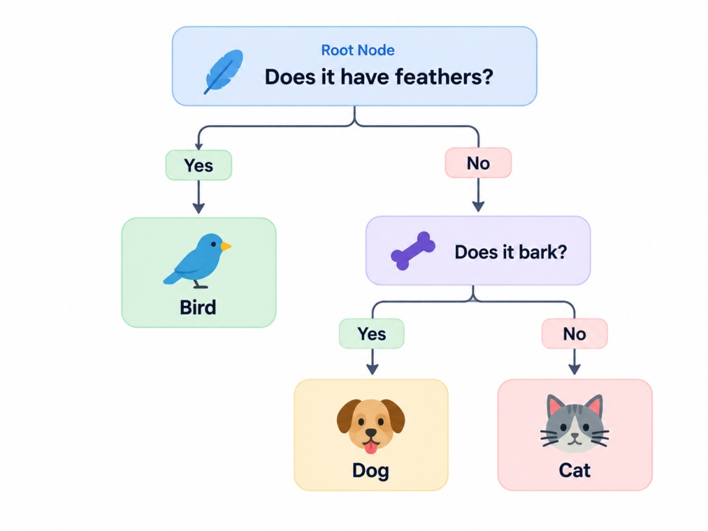
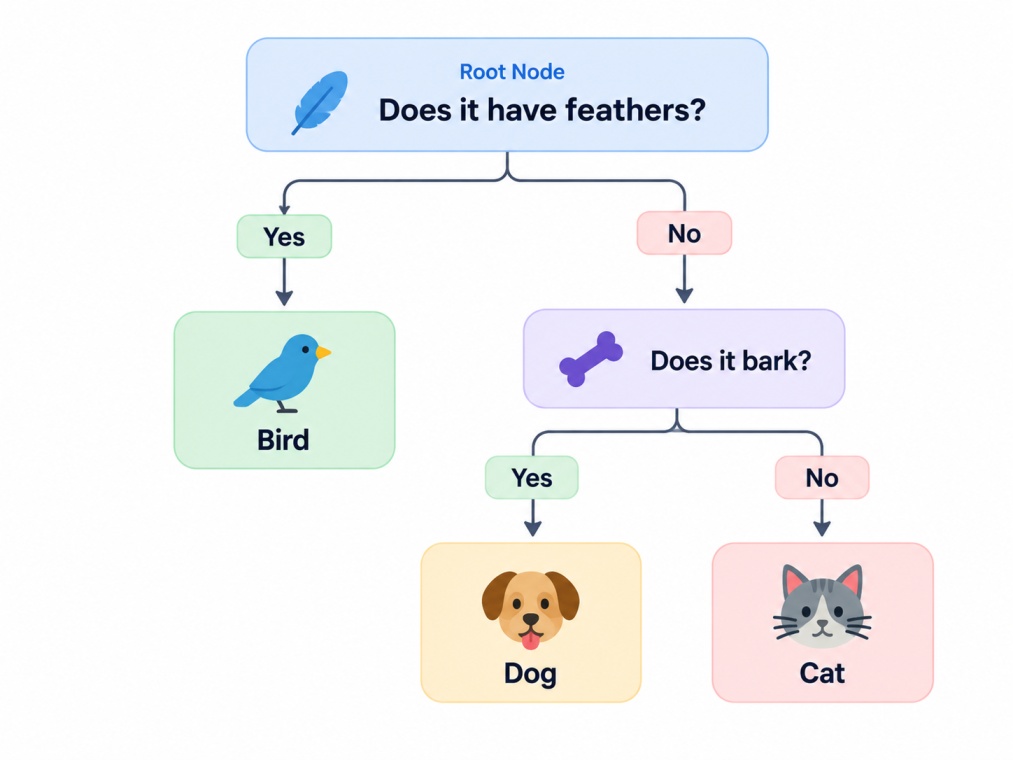
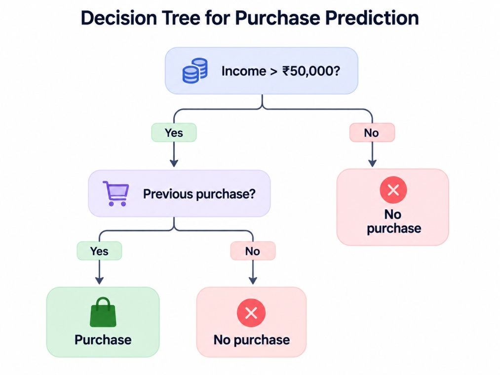
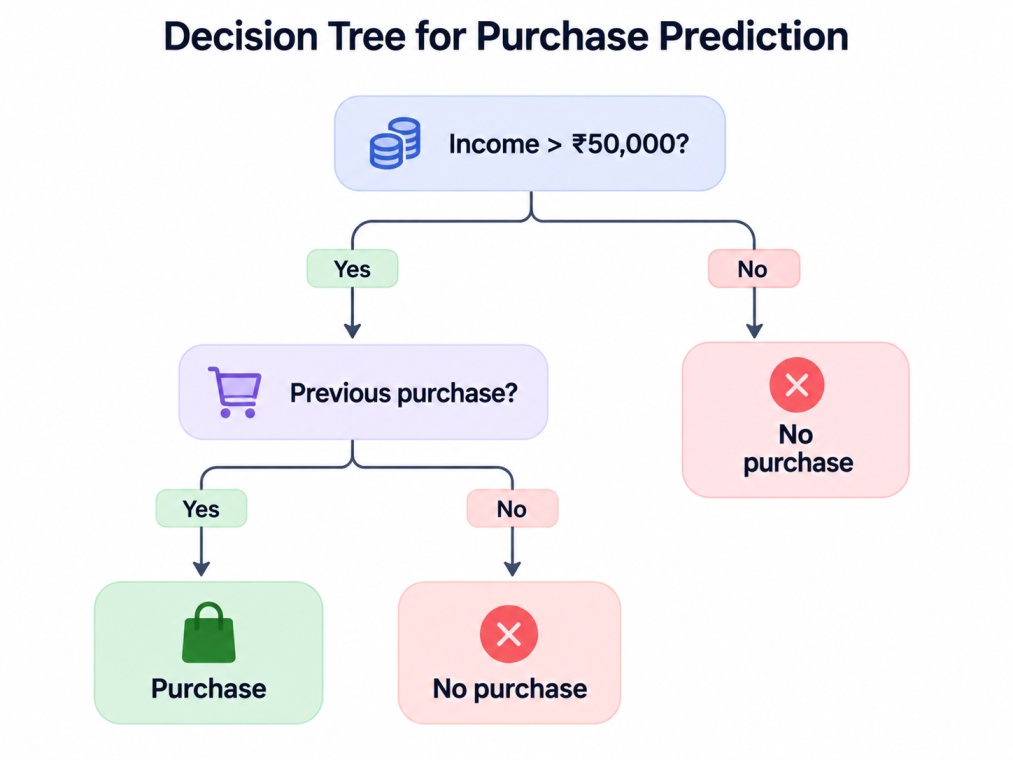
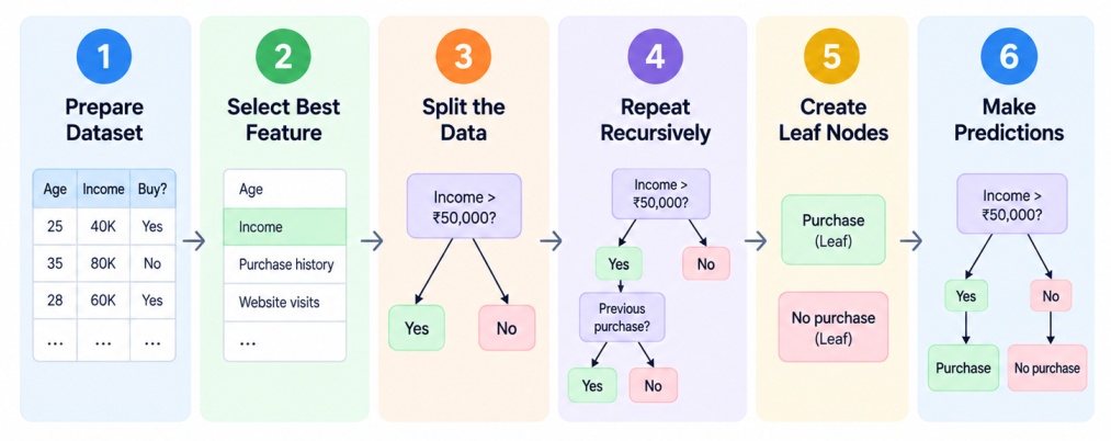
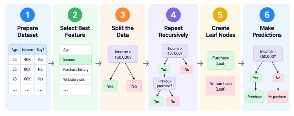
1. Preparing the Dataset
The process starts by preparing the dataset for the training. The labelled training dataset contains one or more independent variables (features) and a dependent variable (the target you want to predict).
For example, a customer dataset might contain:
Age
Income
Purchase history
Website visits
Customer status
The target could be whether the customer makes a purchase.
2. Selecting the Best Feature for Splitting
At the root node, and later at every decision node, the algorithm evaluates every available feature and every possible split point within that feature to find the one that best separates the data into more homogeneous groups.
"Best" here is measured using a splitting criterion, most commonly entropy with information gain, or the Gini index, both covered in detail in the next section.
3. Splitting the Data
After selecting a feature, the algorithm divides the observations according to a condition.
For example:
Age < 30
could divide the dataset into customers below 30 and customers aged 30 or above.
4. Repeating the Splitting Process
The algorithm then repeats the same feature-selection and splitting process independently within each new subset, growing the tree deeper with each round.
This recursive process is what gives tree-based algorithms their name, since each branch effectively becomes a smaller version of the same problem.
5. Creating the Final Leaf Nodes
When further splitting is no longer necessary or a stopping rule is met, the algorithm creates leaf nodes.
Each leaf contains the final prediction for observations that reach that point.
6. Making Predictions
Once the tree is fully built, new observations are predicted by running them down the tree from the root node, following the branch that matches their feature values at each decision node, until they reach a leaf and receive that leaf's stored prediction.
These are the steps which are involved in the decision tree algorithm working process. Now let’s check how a decision tree chooses the best split.
How Does a Decision Tree Choose the Best Split?
One of the most important steps in building a decision tree is choosing an appropriate split. The decision tree algorithm in machine learning uses mathematical measures to determine how effectively a feature separates the target classes.
1. Entropy in Decision Trees
Entropy is a measure of impurity or disorder within a set of data. In the context of a decision tree, it measures how mixed the class labels are in a given node. A node containing only one class has an entropy of 0, meaning it is perfectly pure, while a node with an even mix of classes has higher entropy, closer to its maximum value. The formula for entropy is:
Entropy(S) = -sum(pi * log2(pi))
Where S is the set of data at a given node, and pi is the proportion of examples in S that belong to class i.
For a simple binary classification problem, this simplifies to Entropy(S) = -p1*log2(p1) - p0*log2(p0), where p1 and p0 are the proportions of the positive and negative class respectively.
2. Information Gain
Information gain measures how much a particular split reduces entropy, in other words, how much "purer" the resulting child nodes are compared to the parent node before the split. The formula is:
Information Gain = Entropy(parent) − Weighted Entropy(children)
A feature that produces a larger reduction in entropy provides greater information gain and may be selected as the next splitting feature.
For example, if a dataset has high entropy before a split and much lower entropy after the split, the feature provides useful information for separating the classes.
3. Gini Index
The Gini index, also called Gini impurity, is an alternative measure of impurity that is often used instead of entropy because it is slightly faster to compute, since it avoids the logarithm calculation. Its formula is:
Gini(S) = 1 - sum(pi^2)
Where pi is again the proportion of examples in node S that belong to class i.
Like entropy, a Gini index of 0 means the node is perfectly pure, and the value increases as the class distribution becomes more mixed.
How Is the Best Split Selected?
The algorithm evaluates possible splits and compares their impurity or information gain.
The general selection process include steps such as:
Consider a feature and possible split.
Divide the dataset.
Calculate the resulting impurity or information gain.
Compare it with other possible splits.
Select the split that provides the desired improvement.
Repeat the process for the resulting nodes.
The exact selection process depends on the algorithm and splitting criterion being used.
Gini Impurity vs Entropy
Splitting criterion | What it measures | How it is used | Typical application |
Entropy | Uncertainty or impurity | Uses information gain to select splits | Classification |
Gini impurity | Class impurity | Selects splits that reduce Gini impurity | Classification |
Both can produce effective decision trees. The choice often depends on the implementation and modelling requirements.
Not every decision tree algorithm in machine learning suits every dataset or problem, so choosing the right algorithm is also necessary according to your use case. So now let’s explore what types of decision tree algorithms are available.
Types of Decision Tree Algorithms
Different decision tree algorithms use different methods to select features, create splits, and build the tree. The choice of algorithm depends on the type of problem, dataset, and prediction goal.
1. ID3 (Iterative Dichotomiser 3)
The ID3 algorithm decision tree is one of the early decision tree algorithms, mainly used for classification problems. It selects the feature that provides the highest Information Gain at each step.
Uses entropy to measure uncertainty.
Selects the feature with the highest Information Gain.
Works mainly with categorical features.
Does not handle missing values and continuous data as well as newer algorithms.
Example: An e-commerce company can use ID3 to predict whether a customer will purchase a product based on factors such as age, browsing history, and product category.
2. C4.5
C4.5 is an improved version of the ID3 algorithm decision tree. It was designed to address some of the limitations of ID3 and can work with both categorical and continuous data.
It uses Gain Ratio instead of Information Gain to choose the best split.
Key features include:
Handles continuous variables.
Can work with missing values.
Supports pruning to reduce overfitting.
Mainly used for classification tasks.
3. C5.0
C5.0 is a later version of the C4.5 algorithm. It is designed to build decision trees faster while using less memory, making it suitable for larger datasets.
Its key features include:
Faster training than C4.5.
Supports classification problems.
Handles missing values.
Uses tree pruning to improve predictions.
Can create rule-based models from decision trees.
4. CART (Classification and Regression Trees)
CART is widely used for both classification and regression problems. Unlike some other algorithms, CART creates binary splits, meaning each decision node produces two branches.
For classification, CART commonly uses Gini Impurity to select splits. For regression, it can use measures such as Mean Squared Error (MSE).
Example: CART can classify customers as likely or unlikely to churn, or predict the expected price of a house.
5. CHAID (Chi-square Automatic Interaction Detection)
CHAID uses statistical tests to identify the relationship between input features and the target variable. It can create multiple branches from a single decision node.
It is commonly used for:
Customer segmentation
Market research
Survey analysis
Business decision-making
CHAID is especially useful when you want to understand how different categories of variables are associated with an outcome.
Now, let’s see how to implement a decision tree using Python, because without practical implementation of the decision tree algorithm it becomes difficult to understand the topic in depth.
How to Implement a Decision Tree Classifier in Python?
In this section you will explore a complete decision tree algorithm python example using scikit-learn's DecisionTreeClassifier, predicting whether a loan application is approved based on income, credit score, and existing loans, a simple classification dataset used to demonstrate the complete process end to end.
1. Import the Required Libraries
import numpy as np
import pandas as pd
from sklearn.model_selection import train_test_split
from sklearn.tree import DecisionTreeClassifier, plot_tree, export_text
from sklearn.metrics import accuracy_score, precision_score, recall_score, f1_score, confusion_matrix
import matplotlib.pyplot as plt
2. Load and Prepare the Dataset
np.random.seed(42)
n = 200
income = np.round(np.random.uniform(20000, 120000, n))
credit_score = np.round(np.random.uniform(300, 850, n))
existing_loans = np.random.randint(0, 4, n)
score = (income / 120000) 0.5 + (credit_score / 850) 0.5 - existing_loans * 0.1
approved = ((score + np.random.normal(0, 0.08, n)) > 0.45).astype(int)
df = pd.DataFrame({
"Income": income,
"CreditScore": credit_score,
"ExistingLoans": existing_loans,
"Approved": approved
})
print(df.head())
print(df["Approved"].value_counts())
This creates a sample dataset of 200 loan applications, where approval genuinely depends on income, credit score, and existing loans, with realistic noise layered on top so the relationship is not perfectly clean.
3. Split the Dataset
X = df[["Income", "CreditScore", "ExistingLoans"]]
y = df["Approved"]
X_train, X_test, y_train, y_test = train_test_split(
X, y, test_size=0.2, random_state=42, stratify=y
)
4. Train the Decision Tree Classifier
clf = DecisionTreeClassifier(criterion="gini", max_depth=4, random_state=42)
clf.fit(X_train, y_train)
Setting max_depth=4 here acts as a pre-pruning stopping condition, limiting how deep the tree can grow and helping control overfitting, which is a common and easy first step to take with any decision tree classifier algorithm in scikit-learn.
5. Make Predictions
y_pred = clf.predict(X_test)
6. Evaluate the Model
print("Accuracy:", accuracy_score(y_test, y_pred))
print("Precision:", precision_score(y_test, y_pred))
print("Recall:", recall_score(y_test, y_pred))
print("F1-score:", f1_score(y_test, y_pred))
print("Confusion matrix:\n", confusion_matrix(y_test, y_pred))
Running this example produces an accuracy of roughly 0.80, a precision of roughly 0.79, a recall of roughly 0.86, and an F1-score of roughly 0.83, indicating the model is reasonably good at identifying approved applications, with a slightly higher recall than precision, meaning it is a bit more likely to approve a borderline case than to reject one.
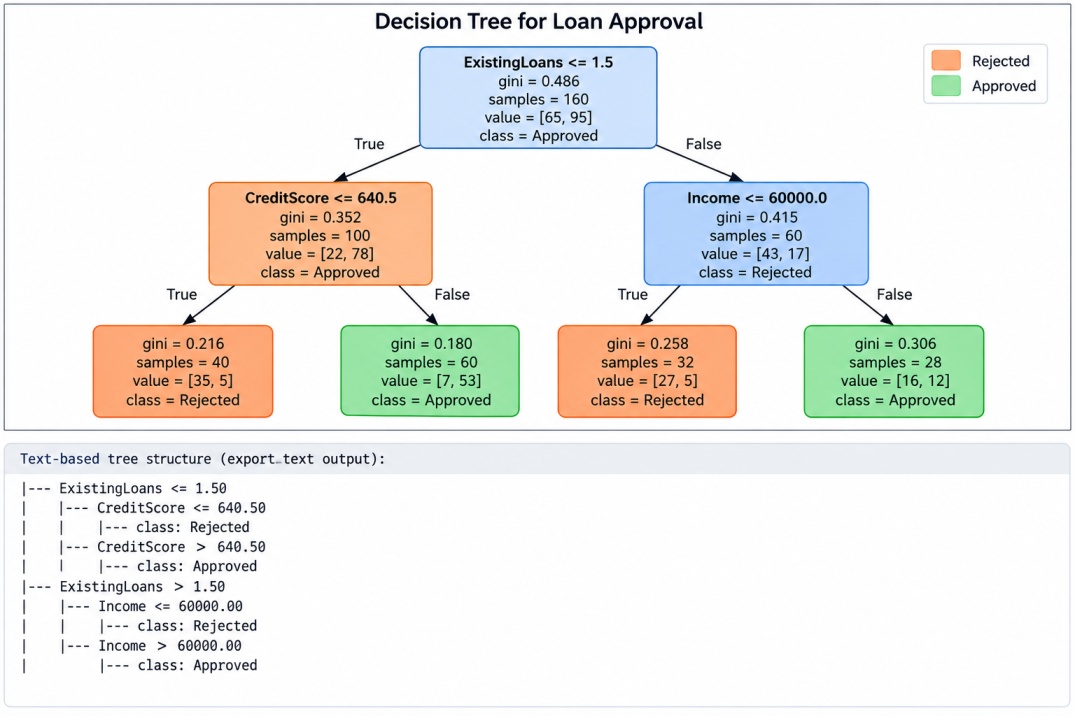
7. Visualise the Decision Tree
plt.figure(figsize=(16, 8))
plot_tree(
clf,
feature_names=X.columns,
class_names=["Rejected", "Approved"],
filled=True,
rounded=True
)
plt.show()
# Alternative: readable text-based tree structure
print(export_text(clf, feature_names=list(X.columns)))
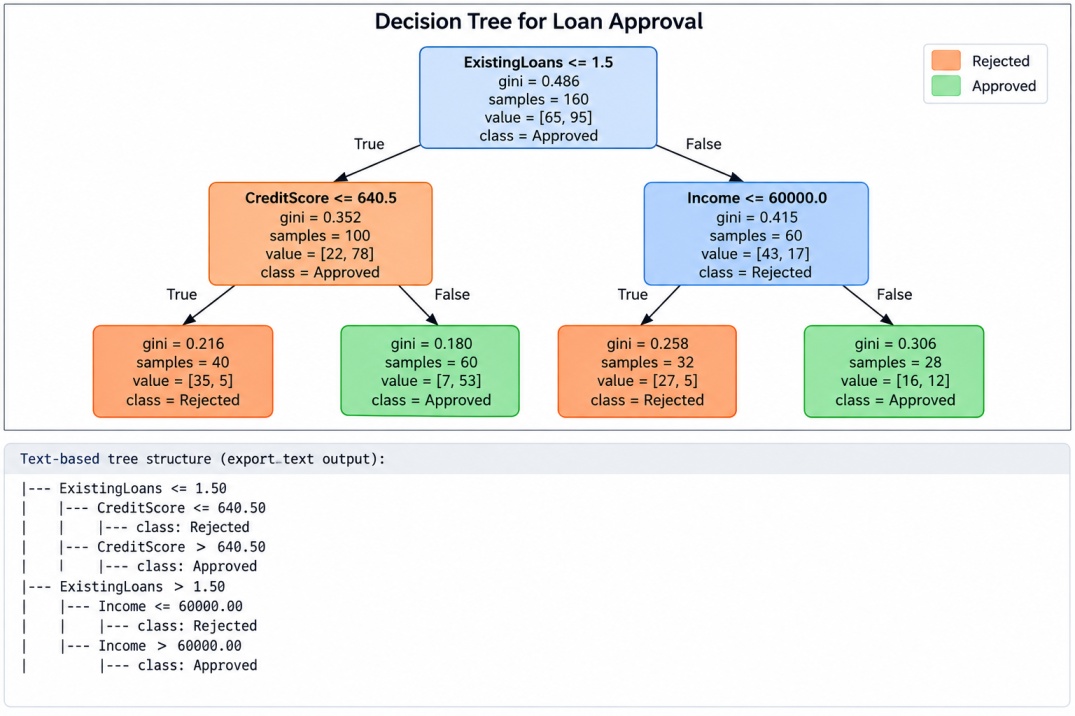
Expected Output: