K Nearest Neighbors Algorithm in Machine Learning: How It Works and Examples

Quick Overview:

• The K Nearest Neighbors algorithm is a supervised machine learning method that predicts outcomes by finding the K closest data points in the training dataset.

• KNN uses distance metrics such as Euclidean and Manhattan distance, while feature scaling helps ensure that larger-valued features do not dominate distance calculations.

• For classification, KNN uses majority voting, while for regression, it generally predicts the average value of the K nearest neighbours.

• In this blog you will learn the KNN algorithm in detail along with its pseudocode, how it works, Python implementation, real-world applications, advantages, disadvantages, and practical examples.

What Is the K Nearest Neighbors Algorithm?

The K nearest neighbors algorithm is a supervised machine learning algorithm which predicts the label or value of the new data point by looking at the K closet data points to its training set and makes predictions on those neighbors. It is used for both classification and regression tasks.

• For classification, the K Nearest Neighbors Algorithm looks at what class those nearby points belong to and then predicts the majority class.

• For regression, it looks at the numerical values of those nearby data points and predicts the average.

Understanding this through a K nearest neighbor algorithm example or analogy is a better way for beginners without being technical from the start. So let’s understand K Nearest Neighbors Algorithm through an analogy:

Imagine you are looking for a new house in a city, and finding out the price of a particular house. Now while searching for the price of that particular house, you would not look for the prices of all houses in the city, you just look for the prices of the houses nearby to the house you are looking for. 

That’s essentially what the K nearest neighbors algorithm in machine learning does with data. For predicting something about a new point, it looks at its nearest neighbor and lets them “vote” or “average out” the answer.

Because it does not build an explicit internal model during training, the K-nearest neighbors algorithm is often described as a “lazy learner.” 

Also Read: Linear Regression in Machine Learning: Types, Algorithm, and Implementation

Now let’s understand this through k nearest neighbor algorithm diagram:

Now let’s take a closer look at some key concepts used in K Nearest Neighbors Algorithm in Machine Learning.

Key Concepts in KNN Algorithm

Before understanding how the K nearest neighbor algorithm works, it is important to understand concepts such as K, distance, distance metrics, and feature scaling.

What Is K in KNN?

K in KNN is simply the number of nearest neighbors the algorithm looks at before making a prediction. If K is set to 5, the algorithm finds the 5 closest points in the training data to the new observation and bases its prediction only on those 5 points, ignoring everything else in the dataset.

Also Read: Supervised vs Unsupervised Learning: Differences, Examples, and Applications

How to Choose the Optimal Value of K in KNN?

Choosing the right value of K in K Nearest Neighbors Algorithm is important because it directly affects model performance.

• Small K: The model becomes more sensitive to individual data points and noise.

• Large K: The model considers more neighbours and produces smoother predictions, but it may overlook local patterns.

• Optimal K: A suitable value balances sensitivity and generalisation.

Why Is Feature Scaling Important in KNN?

Feature scaling is important in KNN because the k nearest neighbor algorithm​ relies entirely on distance calculations to decide which points count as "nearest."

Suppose a dataset contains:

• Age: 18–60

• Income: ₹20,000–₹2,00,000

Income has much larger numerical values than age. Without scaling, income could dominate the distance calculation even if age is equally important.

Techniques such as standardisation or normalisation can bring features to comparable scales before applying k nearest neighbors algorithm​.

Also Read: Logistic Regression in Machine Learning: Algorithm, Types, Examples, and Applications

What Is Distance in KNN?

Distance in KNN is the numeric measure used to determine how "close" two data points are to each other in feature space. Each prediction the algorithm makes depends entirely on correctly measuring this distance between the new observation and every point in the training data, which is why the choice of distance metric, covered below, matters so much to the algorithm's behavior.

How Does KNN Calculate Distance?

The algorithm represents observations as points in a feature space. It then calculates the distance between the new point and existing training points.

For two points:

A = (x₁, x₂)
B = (y₁, y₂)

The distance depends on the selected distance metric. The algorithm calculates the distance from the new observation to the training observations, ranks the distances, and selects the K closest points.

What Are Distance Metrics in KNN?

Distance metrics in K Nearest Neighbors Algorithm are the specific mathematical formulas used to calculate how far apart two points are. Different metrics are used for different kinds of data, and choosing the right one can affect model performance.

1. Euclidean Distance

Euclidean distance is the most commonly used distance metric in k nearest neighbor algorithm in machine learning​, and it corresponds to the straight-line distance between two points, the same distance you would measure with a ruler on a map.

For two points in a two-dimensional space:

d = √[(x₁ − y₁)² + (x₂ − y₂)²]

Where xi and yi are the values of the i-th feature for points x and y.

For example, if:

• A = (2, 3)

• B = (5, 7)

then:

d = √[(2 − 5)² + (3 − 7)²]
d = √(9 + 16)
d = 5

A smaller distance indicates that the two observations are closer to each other.

Also Read: Decision Tree Algorithm in Machine Learning: How It Works, Types, and Examples

2. Manhattan Distance

Manhattan distance, also called taxicab distance, measures the distance between two points by totalling the absolute differences of their coordinates, similar to how a taxi would have to travel along a grid of city blocks rather than cutting diagonally across them. Its formula is:

d = |x₁ − y₁| + |x₂ − y₂|

After understanding these key concepts of k nearest neighbor algorithm in machine learning​ it is now easy to understand its working. But before that let’s explore k nearest neighbor algorithm pseudocode​.

K Nearest Neighbor Algorithm Pseudocode​

The following k nearest neighbor algorithm pseudocode shows the general process for classification and regression.

KNN classification pseudocode:

Given a training dataset with features X and labels y, a value of K, and a new point p:

1. For each point xi in the training dataset:

       Calculate the distance between p and xi using the chosen distance metric

2. Sort all training points by their distance to p, in ascending order

3. Select the K training points with the smallest distance to p

4. Count the class labels among these K nearest neighbors

5. Return the class label that occurs most frequently among the K neighbors

KNN regression pseudocode:

Given a training dataset with features X and target values y, a value of K, and a new point p:

1. For each point xi in the training dataset:

       Calculate the distance between p and xi using the chosen distance metric

2. Sort all training points by their distance to p, in ascending order

3. Select the K training points with the smallest distance to p

4. Return the average of the target values y among these K nearest neighbors

Now after exploring this k nearest neighbor algorithm pseudocode, let’s see how the K Nearest Neighbors Algorithm works.

Also Read: Random Forest Algorithm in Machine Learning: Working, Types, Pseudocode

How Does the K Nearest Neighbors Algorithm Work?

The K nearest neighbors algorithm works by finding the data points that are most similar to a new observation. It calculates the distance between the new point and existing training points, selects the K closest neighbours, and uses their outcomes to make a prediction.

The key steps it follows are:

Step 1: Calculate the Distance

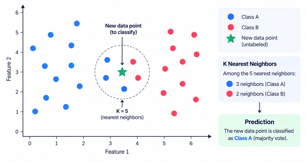
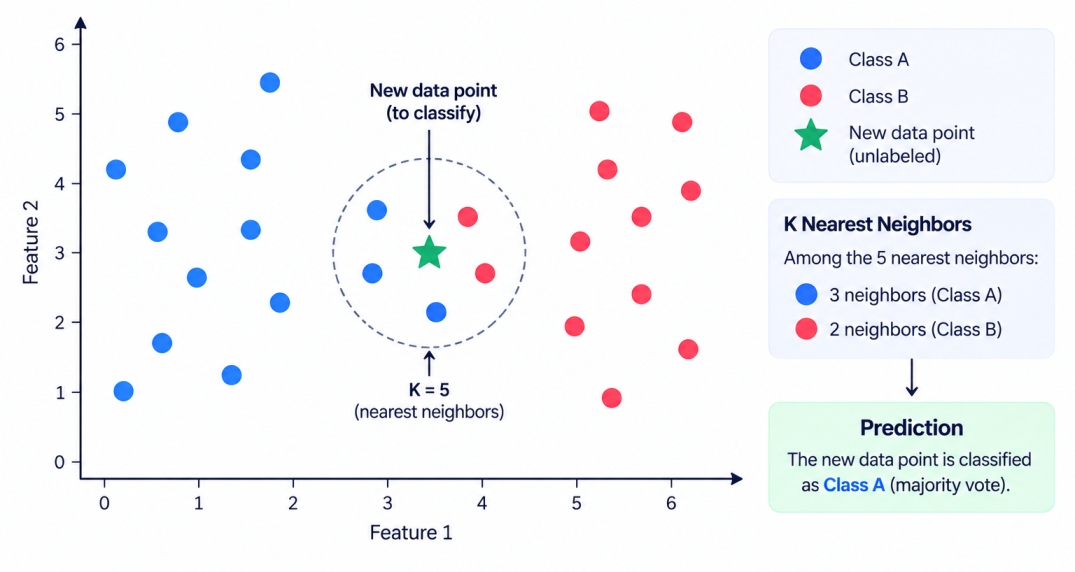
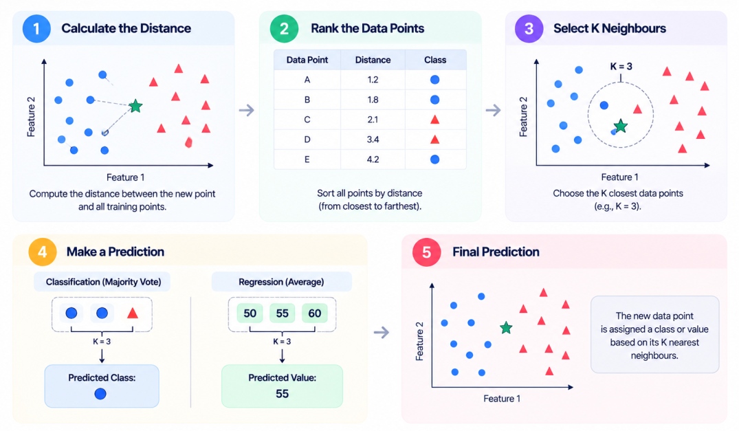
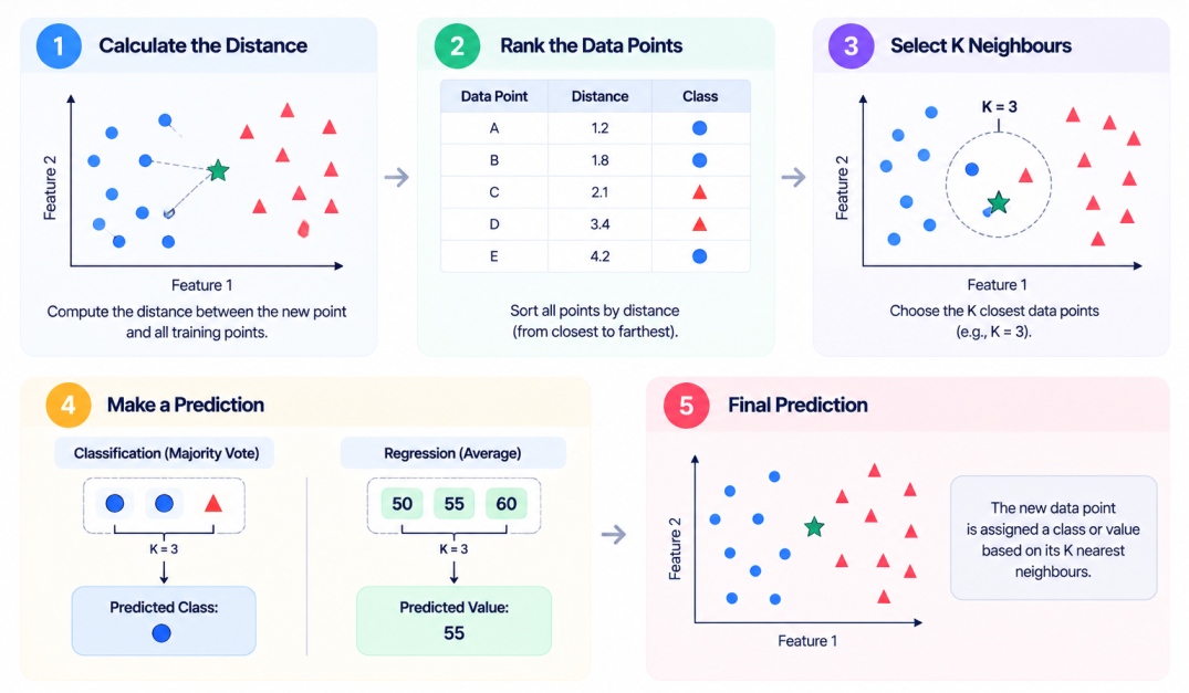
First, it takes a new, unseen data point and calculates the distance between that point and every single point in the training dataset, using a chosen distance metric like Euclidean or Manhattan distance. 

For two data points with multiple features, KNN commonly uses Euclidean distance.

Euclidean Distance = √[(X₁ − Y₁)² + (X₂ − Y₂)² + ... + (Xₙ − Yₙ)²]

For example, consider two points:

• Point A = (5, 7)

• Point B = (2, 3)

Distance = √[(5 − 2)² + (7 − 3)²]

Distance = √[9 + 16] = √25 = 5

Step 2: Rank the Data Points

Once the distances are calculated, KNN sorts the data points from the smallest distance to the largest distance.

For example:

If K = 3, the algorithm selects A, B, and C because they are the three closest points.

Step 3: Make a Classification Prediction

For classification, KNN uses majority voting to determine the predicted class.

Predicted Class = Mode(Class of K Nearest Neighbours)

In the example, the three nearest neighbours are:

• A: Pass

• B: Pass

• C: Fail

Since Pass appears twice, the new data point is classified as Pass.

Step 4: Make a Regression Prediction

For regression, KNN generally calculates the average target value of the K nearest neighbours.

Predicted Value = (y₁ + y₂ + ... + yₖ) / K

For example, if the three nearest properties have prices of ₹50 lakh, ₹55 lakh, and ₹60 lakh:

Predicted Price = (50 + 55 + 60) / 3

Predicted Price = ₹55 lakh

Therefore, KNN predicts the new property's price as ₹55 lakh.

Step 5: Complete the Prediction Process

The overall working of the K nearest neighbor algorithm can be summarised as:

• New Data Point

• Calculate Distance

• Rank Data Points 

• Select K Neighbours

• Vote/Average

• Final Prediction

After exploring the working of the K Nearest Neighbors algorithm, it’s now time to see how the K Nearest Neighbor algorithm can be implemented in Python.

Also Read: Gradient Boosting Algorithm in Machine Learning: How It Works, and Practical Examples

How to Implement KNN in Python

Let’s see the complete k nearest neighbor algorithm python example using scikit-learn, with separate practical examples for KNN classification and KNN regression.

Import Required Libraries

import numpy as np

import pandas as pd

from sklearn.model_selection import train_test_split

from sklearn.preprocessing import StandardScaler

from sklearn.neighbors import KNeighborsClassifier, KNeighborsRegressor

from sklearn.metrics import (

    accuracy_score, precision_score, recall_score, f1_score,

    confusion_matrix, mean_squared_error, r2_score

)

Load and Prepare the Dataset

KNN classification example:

np.random.seed(42)

n = 200

class0 = np.random.normal(loc=[3, 3], scale=1.5, size=(n // 2, 2))

class1 = np.random.normal(loc=[6, 6], scale=1.5, size=(n // 2, 2))

X = np.vstack([class0, class1])

y = np.array([0] (n // 2) + [1] (n // 2))

df = pd.DataFrame(X, columns=["Feature1", "Feature2"])

df["Label"] = y

print(df.head())

This creates two overlapping clusters of 100 points each, a simple k nearest neighbor algorithm example used to demonstrate binary classification.

Split the Data

X_train, X_test, y_train, y_test = train_test_split(

    X, y, test_size=0.2, random_state=42, stratify=y

)

Scale the Features

scaler = StandardScaler()

X_train_scaled = scaler.fit_transform(X_train)

X_test_scaled = scaler.transform(X_test)

As covered earlier, scaling is essential for KNN specifically, since the algorithm's predictions are based entirely on distance calculations that can be distorted by features on different numeric scales.

Train the KNN Model

clf = KNeighborsClassifier(n_neighbors=5)

clf.fit(X_train_scaled, y_train)

Setting n_neighbors=5 means the model will look at the 5 nearest training points whenever it makes a prediction, consistent with the value of K covered earlier in this guide.

Make Predictions

y_pred = clf.predict(X_test_scaled)

Evaluate the Model

print("Accuracy:", accuracy_score(y_test, y_pred))

print("Precision:", precision_score(y_test, y_pred))

print("Recall:", recall_score(y_test, y_pred))

print("F1-score:", f1_score(y_test, y_pred))

print("Confusion matrix:\n", confusion_matrix(y_test, y_pred))

Running this classification example produces an accuracy of roughly 0.975, a precision of 1.0, a recall of roughly 0.95, and an F1-score of roughly 0.97, showing the model correctly separates the two clusters with only a single misclassification in the test set.

KNN regression example, predicting house price from size, bedrooms, and age:

np.random.seed(7)

size = np.round(np.random.uniform(500, 3500, n))

bedrooms = np.random.randint(1, 5, n)

age = np.round(np.random.uniform(0, 30, n))

price = 20000 + size 120 + bedrooms 8000 - age * 500 + np.random.normal(0, 15000, n)

df_house = pd.DataFrame({"Size": size, "Bedrooms": bedrooms, "Age": age, "Price": price})

X_reg = df_house[["Size", "Bedrooms", "Age"]]

y_reg = df_house["Price"]

X_train_r, X_test_r, y_train_r, y_test_r = train_test_split(

    X_reg, y_reg, test_size=0.2, random_state=42

)

scaler_r = StandardScaler()

X_train_r_scaled = scaler_r.fit_transform(X_train_r)

X_test_r_scaled = scaler_r.transform(X_test_r)

reg = KNeighborsRegressor(n_neighbors=5)

reg.fit(X_train_r_scaled, y_train_r)

y_pred_r = reg.predict(X_test_r_scaled)

mse = mean_squared_error(y_test_r, y_pred_r)

rmse = np.sqrt(mse)

r2 = r2_score(y_test_r, y_pred_r)

print("RMSE:", rmse)

print("R2 score:", r2)

On this regression example, the model achieves an R² score of roughly 0.93 and an RMSE of roughly 29,600, meaning it explains about 93 percent of the variance in house price and its predictions are typically off by around that RMSE amount, a solid result for a simple, untuned KNN regressor.

Also Read: Support Vector Machine (SVM) in Machine Learning: Algorithm, Types, Kernels, and Examples

Real world applications of K Nearest Neighbors Algorithm tells how it is applied in various use cases, and helps to understand the algorithm more clearly. Let’s explore some of the applications of k nearest neighbor algorithm in machine learning​.

Applications of K Nearest Neighbors Algorithm in Real-World 

The K nearest neighbors algorithm can be applied to several classification and regression problems where similarity between observations is useful. 

Some key applications of K Nearest Neighbors Algorithm are:

Now that we have explored the applications of the K Nearest Neighbors Algorithm, let’s take a look at the k nearest neighbor algorithm advantages and disadvantages to understand its strengths and limitations.

Advantages and Disadvantages of K Nearest Neighbors Algorithm

Like every machine learning technique, KNN has strengths and weaknesses. Understanding these can help you to determine whether it is suitable for your particular problem or not.

Advantages of K Nearest Neighbors Algorithm

1. Simple to understand: The algorithm follows an intuitive similarity-based approach.

2. Easy to implement: K Nearest Neighbors Algorithm can be implemented with relatively little code using machine learning libraries.

3. No complex training process: It does not require learning a complex set of model parameters during training.

4. Works for classification and regression: KNN can solve both categorical and numerical prediction problems.

5. Flexible decision boundaries: KNN can capture nonlinear relationships because predictions are based on local observations.

Disadvantages of K Nearest Neighbors Algorithm

1. Prediction can be computationally expensive: The algorithm may need to calculate distances to many training observations.

2. Sensitive to feature scaling: Features with larger numerical ranges can dominate distance calculations.

3. Sensitive to the choice of K: A poorly selected K can lead to underfitting or overfitting.

4. Affected by irrelevant features: Unimportant variables can distort distance calculations.

5. Performance can decline with high-dimensional data: As the number of features increases, identifying meaningful nearest neighbours can become more difficult.

Conclusion

So far, you have learned that the K Nearest Neighbors algorithm remains a valuable tool in machine learning because it closely mirrors human intuition. When predicting something about a new observation, it looks at what similar observations can already tell us.

Understanding K, distance metrics, feature scaling, and the lazy learning approach behind KNN gives a strong foundation for using it effectively, whether for classification, regression, or as a reliable baseline before moving on to more complex algorithms.