Logistic Regression in Machine Learning: Algorithm, Types, Examples, and Applications

Quick Overview:

• Logistic regression in machine learning is a supervised learning algorithm used to predict the probability of categorical outcomes, particularly in classification problems.

• The model uses a sigmoid function to convert input values into probabilities between 0 and 1, which are then converted into class predictions using a threshold.

• Binary, multinomial, ordinal, and Bayesian logistic regression are the main types, used for different classification problems and target categories.

• This blog covers logistic regression in detail along with sigmoid function, evaluation metrics, assumptions, applications, advantages and disadvantages, and implementation of logistic regression with Python.

What Is Logistic Regression in Machine Learning?

Logistic regression is the most widely used supervised machine learning algorithm, used for binary classification tasks.  It is used to predict the probability of a categorical outcome, meaning when there are two possible outcomes such as yes/no, pass/fail etc. it is mostly used.

Instead of directly predicting a class, the logistic regression algorithm in machine learning​ first calculates a probability between 0 and 1. A probability threshold is then used to assign the observation to a class.

Suppose, If a bank wants to predict that a particular customer will pay the loan on time or it will default.  The model uses factors such as income, credit history, loan amount, and repayment history to calculate the probability of default.

If the predicted probability of default is above the threshold, the customer may be classified as a defaulter; otherwise, it may be classified as a non-defaulter.

Why Is Logistic Regression Used for Classification?

Logistic regression in machine learning is used for classification because its output is between 0 and 1, so it can represent a probability.

A straight-line model could produce values below 0 or above 1, which cannot be probabilities. The sigmoid function solves this by converting any input into a value between 0 and 1. This output can then be interpreted as the probability that an observation belongs to the positive class.

For a binary classification problem:

• Probability close to 1: more likely to belong to the positive class

• Probability close to 0: more likely to belong to the negative class

For example, if the model predicts an 0.82 probability that an email is spam and the threshold is 0.5, the email is classified as spam.

Logistic regression is also easy to understand because its coefficients show how changes in input variables affect the predicted outcome.

If you are now confused about the difference between straight-line model and classification. So, let’s explore some key differences between linear and logistic regression in machine learning​.

Difference Between Linear and Logistic Regression in Machine Learning

Linear and logistic regression in machine learning are both supervised learning algorithms, but they solve different types of prediction problems.

For example, predicting a person's salary is generally a regression problem, while predicting whether the person will leave a company is a classification problem. 

Now let’s explore how logistic regression in machine learning works, which helps you to understand the topic more clearly.

How Does the Logistic Regression Algorithm in Machine Learning Work?

The logistic regression algorithm learns coefficients for each input variable and an intercept to make the best possible probability predictions on the training data. 

The key steps involved in the working on logistic regression algorithm are:

1. Collect labelled training data: Gather data where each observation already has a known class or outcome, such as spam or not spam.

2. Select relevant features and the target variable: Choose the input variables (features) that will be used to predict the target class.

3. Calculate a weighted combination of the features: The model multiplies each feature by a learned coefficient and adds them together with an intercept.

4. Pass the result through the sigmoid function: The weighted result is passed through the sigmoid function, which converts it into a value between 0 and 1.

5. Obtain a probability: The output is interpreted as the probability that the observation belongs to the positive class.

6. Apply a classification threshold: A threshold, commonly 0.5, is used to decide which class the observation belongs to.

7. Assign the observation to a class: If the probability is ≥ 0.5, it is assigned to the positive class; otherwise, it is assigned to the negative class.

The working of logistic regression in machine learning follows these key steps. If you are confused with the terms such as Sigmoid Function, Cost Function; do not worry as now you will explore each of them in detail.

1. Logistic Regression Equation and Formula

The logistic regression in machine learning formula is based on the odds and log-odds of the predicted probability.

First, the linear combination of features is calculated as:

z = β₀ + β₁x₁ + β₂x₂ + ... + βₙxₙ

The predicted probability is then:

P(Y = 1 | X) = 1 / (1 + e⁻ᶻ)

Where:

• P(Y = 1 | X) = probability of the positive class

• β₀ = intercept

• β₁, β₂, ..., βₙ = model coefficients

• x₁, x₂, ..., xₙ = input features

• e = Euler's number

• z = weighted sum of the input variables

For example, if:

z = 2

Then:

P(Y = 1) = 1 / (1 + e⁻²)

P(Y = 1) ≈ 0.881

Therefore, the model estimates an approximately 88.1% probability of belonging to the positive class.

2. What Is the Sigmoid Function?

The sigmoid function converts any number into a value between 0 and 1, which makes it suitable for representing a probability.

Its formula is:

σ(z) = 1 / (1 + e⁻ᶻ)

When z is very positive, the sigmoid output approaches 1. When z is very negative, the output approaches 0.

For example:

3. Cost Function in Logistic Regression

The cost function measures how well a logistic regression model predicts the actual class labels.

Logistic regression in machine learning commonly uses log loss, also called binary cross-entropy, for binary classification.

The formula is:

J(β) = −1/n Σ [yᵢ log(pᵢ) + (1 − yᵢ) log(1 − pᵢ)]

Where:

• n = number of observations

• yᵢ = actual class

• pᵢ = predicted probability

The model aims to minimise this cost. Wrong predictions with high confidence receive a larger penalty, while predictions closer to the correct probability receive a smaller penalty.

The next step is to understand the types of logistics regression in machine learning. 

Types of Logistic Regression in Machine Learning

Logistic regression can be classified based on the number and nature of the target classes. The main types of logistic regression algorithms in machine learning are:

1. Binary Logistic Regression

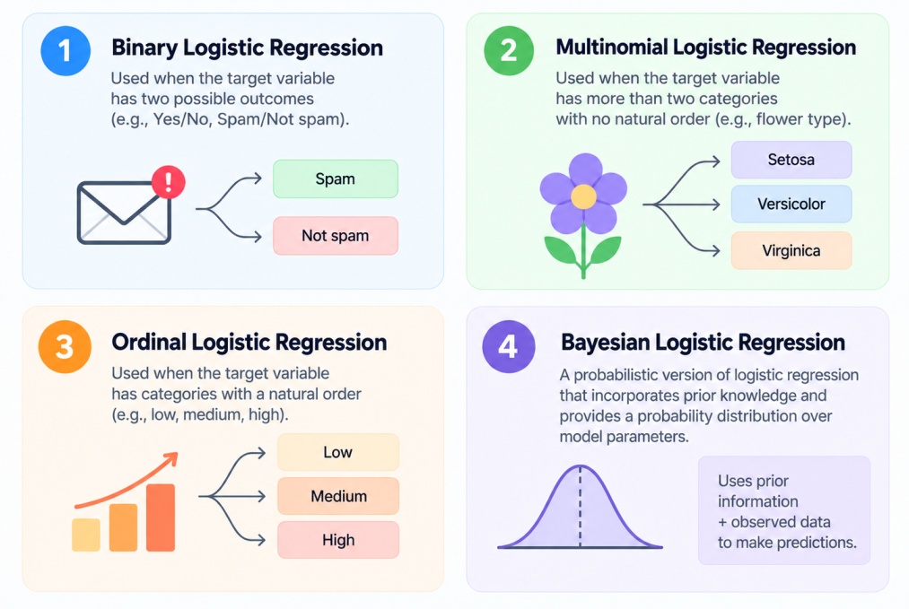
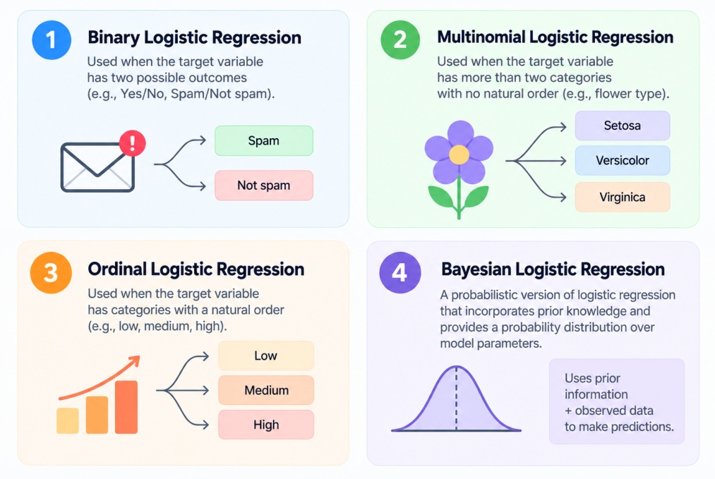
Binary logistic regression is a statistical method used to predict the probability of an outcome with two possible classes, commonly represented as 0 or 1.

Examples include:

• Spam or not spam

• Pass or fail

• Churn or no churn

• Disease or no disease

• Default or no default

For example, a healthcare model can predict whether a patient has a disease or not:

0 = No disease

1 = Disease

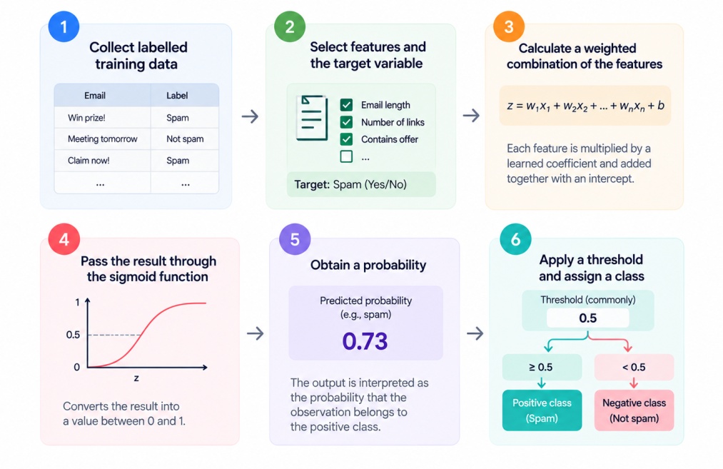
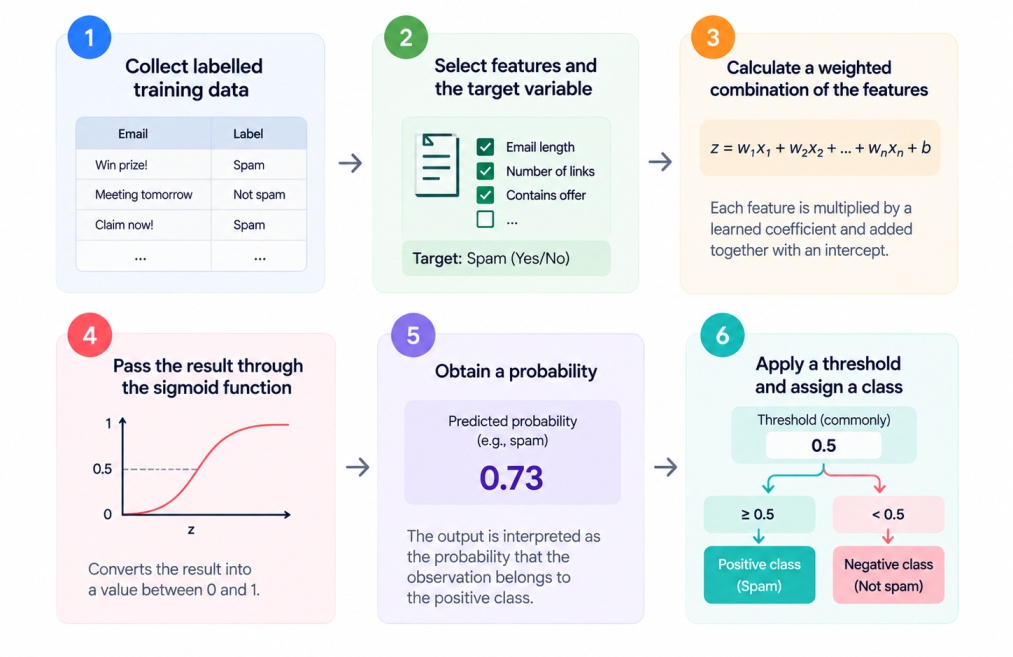
The model produces a probability, which can then be converted into one of the two classes using a threshold.

2. Multinomial Logistic Regression

Multinomial logistic regression in machine learning is used when the target variable has three or more categories with no natural order. 

For example, a customer might be classified according to their preferred product category:

• Electronics

• Clothing

• Grocery

• Furniture

The model estimates the probability of each possible class and assigns the observation to the class with the highest probability or based on a selected decision rule.

3. Ordinal Logistic Regression

Ordinal logistic regression in machine learning is used when the target variable has three or more categories that follow a natural order. Unlike multinomial categories, ordinal classes have a clear natural ranking. This makes ordinal logistic regression useful when the order of the outcomes is important.

For example, customer satisfaction could be classified as:

• Low 

• Medium 

• High 

4. Bayesian Logistic Regression

Bayesian logistic regression estimates coefficients by treating them as probability distributions instead of single values. 

It uses prior information and updates it with new data. This provides both predictions and a measure of uncertainty, which is useful when understanding the confidence of a prediction is important. 

For example, medical researchers can use Bayesian logistic regression in machine learning to predict whether a patient is at risk of developing a disease.

The model can predict a 75% probability of disease, along with an uncertainty range. This helps researchers understand both the predicted risk and how confident the model is in that prediction.

How to Evaluate a Logistic Regression Model?

Logistic regression in machine learning predicts categories rather than continuous numbers, so it is evaluated with a different set of metrics than linear regression, most of which are built from a single table called the confusion matrix.

1. Accuracy

Accuracy measures the percentage of predictions that are correctly classified. It works well when the classes are fairly balanced and different types of errors have similar importance.

Accuracy = (TP + TN) / (TP + TN + FP + FN)

Where:

• TP = True Positives

• TN = True Negatives

• FP = False Positives

• FN = False Negatives

2. Precision

Precision measures how many of the observations predicted as positive are really positive.

Precision = TP / (TP + FP)

For example, precision is important in spam detection when you want to minimize legitimate emails being incorrectly classified as spam.

3. Recall

Recall, also called sensitivity, measures how many of the actual positive cases are correctly identified by the model. 

It is especially important when missing a positive case could have serious consequences, such as failing to detect a serious disease.

Recall = TP / (TP + FN)

4. F1-Score

The F1-score combines precision and recall into a single number using their harmonic mean:

F1 = 2 × (Precision × Recall) / (Precision + Recall)

The F1-score is useful when you need a balance between precision and recall, particularly on imbalanced datasets where accuracy alone would give a misleadingly optimistic picture of model performance.

5. Confusion Matrix

A confusion matrix provides a table showing the number of:

• True positives

• True negatives

• False positives

• False negatives

Accuracy, precision, recall, and F1-score are all calculated using these values, making it a useful starting point for evaluating a logistic regression model.

6. ROC-AUC

• The Receiver Operating Characteristic (ROC) curve shows how the true positive rate and false positive rate change at different classification thresholds.

• The Area Under the Curve (AUC) summarises the model's ability to distinguish between the classes. A higher AUC generally indicates better class-separation ability.

How to Choose a Probability Threshold?

A logistic regression model produces probabilities, and a threshold is used to convert them into class predictions.

A common starting point is 0.5:

• Probability ≥ 0.5 → Class 1

• Probability < 0.5 → Class 0

However, 0.5 is not always the best threshold. The appropriate value depends on the cost of false positives and false negatives.

For example, a healthcare screening model may use a lower threshold to improve recall and reduce missed positive cases.

Now let's look at some of the assumptions used in logistic regression in machine learning.

Assumptions of Logistic Regression in Machine Learning

Logistic regression in machine learning has fewer assumptions than linear regression. It does not require normally distributed residuals or equal variance, but some important assumptions still need to be met for the model to give reliable results.

1. Independent Observations

Each observation should be independent of the others. If observations are strongly related, the model’s results may become unreliable.

This is especially important with repeated measurements, grouped data, or time-based data.

2. Linear Relationship Between Predictors and Log-Odds

Logistic regression in machine learning does not require a linear relationship between the predictor and the probability. Instead, it assumes a linear relationship between the predictors and the log-odds of the outcome.

If this assumption is not met, transformations or additional features may be needed.

3. Absence of Multicollinearity

Independent variables should not be highly correlated with each other. High correlation can make the model’s coefficients unstable and make it difficult to understand the effect of each variable.

Correlation analysis and measures such as Variance Inflation Factor (VIF) can be used to detect multicollinearity.

4. Appropriate Sample Size

Logistic regression generally requires enough observations and sufficient examples of each outcome class to estimate the model reliably.

Very small datasets or datasets with extremely rare positive outcomes can lead to unstable estimates.

How to Check Logistic Regression Assumptions?

You can check assumptions using:

• Correlation matrices

• VIF

• Scatter plots and feature analysis

• Residual and diagnostic analysis

• Class-distribution checks

• Cross-validation

• Model performance on unseen data

These checks help identify issues before using the model for predictions or business decisions.

How to Implement Logistic Regression in Python

In this section you will explore full logistic regression in machine learning python code example and a logistic regression in machine learning python implementation using scikit-learn, predicting whether a student passes a course based on hours studied and class attendance, a simple and intuitive binary classification example.

1. Preparing the Dataset

import numpy as np

import pandas as pd

from sklearn.model_selection import train_test_split

from sklearn.preprocessing import StandardScaler

from sklearn.linear_model import LogisticRegression

from sklearn.metrics import (

    accuracy_score, precision_score, recall_score,

    f1_score, confusion_matrix, roc_auc_score

)

np.random.seed(42)

n = 200

hours_studied = np.round(np.random.uniform(0, 10, n), 1)

attendance = np.round(np.random.uniform(50, 100, n), 1)

# Simulate a realistic pass/fail outcome using a true logistic relationship

z = -8 + 0.9 hours_studied + 0.05 attendance

prob = 1 / (1 + np.exp(-z))

passed = np.random.binomial(1, prob)

df = pd.DataFrame({

    "HoursStudied": hours_studied,

    "Attendance": attendance,

    "Passed": passed

})

print(df.head())

print(df["Passed"].value_counts())

This creates a sample dataset of 200 students, where the probability of passing genuinely depends on hours studied and attendance through a logistic relationship, with realistic randomness layered on top.

2. Selecting Features and Target Variables

X = df[["HoursStudied", "Attendance"]]

y = df["Passed"]

Here, HoursStudied and Attendance are the independent variables, and Passed is the binary target variable the model will learn to predict.

3. Splitting Data Into Training and Test Sets

X_train, X_test, y_train, y_test = train_test_split(

    X, y, test_size=0.2, random_state=42, stratify=y

)

Using stratify=y keeps the proportion of passed and failed students consistent between the training and test sets, which matters more in classification problems than in regression, especially when classes are not perfectly balanced.

4. Training the Logistic Regression Model

scaler = StandardScaler()

X_train_scaled = scaler.fit_transform(X_train)

X_test_scaled = scaler.transform(X_test)

model = LogisticRegression()

model.fit(X_train_scaled, y_train)

print("Intercept:", model.intercept_)

print("Coefficients:", model.coef_)

Scaling the input features before training is a common practice in logistic regression, since it helps the gradient-based optimiser used internally converge faster and makes the resulting coefficients more directly comparable to each other.

5. Making Predictions

y_pred = model.predict(X_test_scaled)

y_prob = model.predict_proba(X_test_scaled)[:, 1]

model.predict returns the final class label using the default 0.5 threshold, while model.predict_proba returns the actual predicted probability, which is useful if you want to apply a custom threshold instead.

6. Evaluating the Model

print("Accuracy:", accuracy_score(y_test, y_pred))

print("Precision:", precision_score(y_test, y_pred))

print("Recall:", recall_score(y_test, y_pred))

print("F1-score:", f1_score(y_test, y_pred))

print("Confusion matrix:\n", confusion_matrix(y_test, y_pred))

print("ROC-AUC:", roc_auc_score(y_test, y_prob))

Running this full example produces an accuracy of roughly 0.83, a precision of roughly 0.89, a recall of roughly 0.77, an F1-score of roughly 0.83, and a ROC-AUC of roughly 0.92. 

Together, these numbers suggest the model is quite good at distinguishing passing from failing students, with slightly stronger precision than recall, meaning it is a little more likely to miss a genuine pass than to incorrectly predict one.

Applications of Logistic Regression in Machine Learning

Logistic regression in machine learning is widely used for classification problems where the outcome belongs to one or more categories.

Most common applications include: 

Till now the linear regression algorithm in machine learning is mostly clear. Let’s look at some advantages and disadvantages of Logistic Regression.

Advantages and Disadvantages of Logistic Regression in Machine Learning

Logistic regression in machine learning is a strong fit for many classification problems but not a universal solution, so let’s look at the advantages and disadvantages of logistic regression in machine learning before committing to it for a given dataset.

Advantages of Logistic Regression in Machine Learning

Some key advantages include:

• Simple to implement and understand

• Fast to train

• Computationally efficient

• Produces probability estimates

• Coefficients are relatively interpretable

• Works well as a classification baseline

• Supports regularisation

• Suitable for high-dimensional datasets with appropriate feature selection

Disadvantages of Logistic Regression in Machine Learning

Despite its benefits, logistic regression has limitations:

• Assumes a linear relationship with the log-odds

• Can struggle with highly non-linear relationships

• Sensitive to multicollinearity

• Can be affected by outliers and influential observations

• May perform poorly when classes are not well separated

• Imbalanced datasets can distort accuracy

• Complex relationships may require feature engineering

When Logistic Regression May Not Be Suitable

Logistic regression may not be the best choice when:

• The relationship between predictors and log-odds is strongly non-linear.

• The dataset contains complex interactions.

• Classes have highly irregular decision boundaries.

• The dataset contains severe multicollinearity.

• More complex models can provide substantial performance improvements.

In such cases, algorithms such as decision trees, random forests, support vector machines, or neural networks may be considered.

Conclusion

Logistic regression in machine learning is a simple and interpretable algorithm for classification problems. It uses probability, the sigmoid function, and a decision threshold to classify outcomes effectively.

Understanding its types, evaluation metrics, assumptions, Python implementation, and common challenges can help you build reliable classification models and choose logistic regression when it fits your data and objectives.