Gradient Boosting Algorithm in Machine Learning: How It Works, and Practical Examples

Quick Overview:

• The gradient boosting algorithm builds a strong predictive model by combining multiple weak decision trees sequentially, with each new tree learning from the errors of the previous models.

• It uses concepts such as weak learners, loss functions, gradient descent, learning rate, number of estimators, and tree depth to progressively improve model performance.

• Algorithms such as GBDT, AdaBoost, XGBoost, LightGBM, and CatBoost use different approaches to improve prediction performance, speed, or handling of specific data types.

• In this blog you will explore gradient boosting algorithms in detail along with its types, applications, pros and cons, examples and comparisons with methods such as random forest, XGBoost, LightGBM, and CatBoost.

What Is the Gradient Boosting Algorithm?

The gradient boosting algorithm is a supervised machine learning technique that builds a strong predictive model by combining many simple models, usually small decision trees, in sequence.  

Each new tree is trained to predict the errors, or residuals, left behind by the combination of all the trees built before it, and its predictions are added to the ensemble to gradually reduce the overall error. Over many rounds, this sequential correction process produces a final model that is often considerably more accurate than any single tree, and frequently more accurate than a random forest.

Let’s understand gradient boosting algorithms by a simple analogy:

Imagine you are preparing for an exam, in which a team of tutors is helping you.

• The first tutor looks at your answers and gives you a rough prediction.

• You check the mistakes you made.

• The second tutor focuses specifically on those mistakes and tries to correct them.

• Then you check what's still wrong.

• The third tutor focuses on the remaining errors.

• This continues, with each tutor improving what the previous tutors got wrong.

In gradient boosting, each tutor is like a small decision tree. The new tree doesn't start from scratch, it learns from the errors (residuals) made by the existing collection of trees.

Now let’s explore what are the gradient boosted trees to understand the gradient boosted trees algorithm​ more clearly.

What Are Gradient-Boosted Trees?

Gradient-boosted trees are decision trees used as the weak learners in a gradient boosting model. These trees are generally kept relatively small so that each one makes a limited contribution to the final prediction.

Instead of depending on one complex decision tree, the model combines many smaller trees. Each tree is trained after the previous one and attempts to improve the overall ensemble.

It is also important to understand how gradient boosting is different from the decision tree. So, now explore the difference between both.

Gradient Boosting vs Decision Trees

A traditional decision tree makes predictions using a single tree. Gradient boosting, on the other hand, combines many trees and trains them sequentially.

By looking at how the gradient boosting algorithm works in machine learning, it will be easier to understand the topic. So, let’s take a look at how it works.

How Does Gradient Boosting Work?

The gradient boosting algorithm follows a sequential process in which every new model attempts to improve the performance of the existing ensemble. 

It follow these six step process:

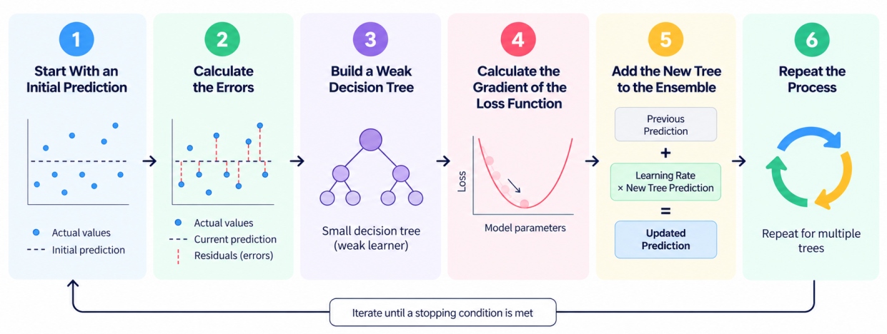
Step 1: Start With an Initial Prediction

The algorithm starts with a simple initial prediction that acts as the baseline.

• For a regression problem, this may be based on a central value of the target, such as the mean for common squared-error loss. 

• For classification, the initial model depends on the selected loss function and target structure.

The initial predictions will generally contain errors. These errors provide the information needed for the next stage.

Step 2: Calculate the Errors

The gradient boosting algorithm​ compares the actual target values with the current model's predictions.

For a simple regression example:

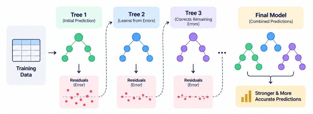
The residual represents the difference between what the model predicted and the actual value. The next tree is trained to learn these remaining errors rather than starting from the original target values again.

Step 3: Build a Weak Decision Tree

The algorithm trains a new and small decision tree to record the patterns in the current errors or, more generally, the direction that would reduce the selected loss function.

This tree is called a weak learner because it is intentionally limited in complexity.

The goal is not for one tree to solve the entire problem. Instead, each tree makes a small improvement to the existing ensemble.

Step 4: Calculate the Gradient of the Loss Function

A loss function is a mathematical measure of how far the model's current predictions are from the actual target values, similar in role to the cost functions used in linear and logistic regression.

Gradient boosting uses the gradient of the loss function to determine how the model should improve its predictions.

The gradient indicates the direction in which the loss can be reduced. The next tree is therefore trained to approximate these negative gradients, often referred to as pseudo-residuals. This is where the term "gradient" in gradient boosting comes from.

Step 5: Add the New Tree to the Ensemble

Once the new tree is trained, its predictions are added to the existing model. However, the tree's contribution is controlled using a learning rate, also called shrinkage.

A simplified update can be represented as:

New Prediction = Previous Prediction + Learning Rate × New Tree Prediction

A smaller learning rate means each tree contributes less to the final prediction. The model may then require more trees to achieve strong performance.

Step 6: Repeat the Process

The algorithm repeats the process:

Predict → Calculate Loss/Gradient → Train Tree → Update Predictions

• Each new tree attempts to improve the errors remaining after the previous iterations.

• The process continues until a predefined number of estimators is reached or another stopping condition, such as early stopping, is triggered.

• The number of estimators determines how many boosting iterations are performed. Too few trees can result in underfitting, while too many can increase the risk of overfitting if other controls are not used.

If you are confused about the terms such as loss function, weak learner etc. Do not worry it is common for beginners while exploring the working. So now let’s see all these concepts in detail.

Key Concepts Behind Gradient Boosting

There are several important concepts that determine how a gradient boosting model learns and performs. 

1. Weak Learners

A weak learner is a simple model that performs better than random guessing but is not expected to solve the entire prediction problem independently.

In gradient boosting, shallow decision trees commonly serve as weak learners. Each tree focuses on improving the existing ensemble.

2. Loss Function

A loss function is used to measure the difference between predicted and actual values.

The choice of loss function depends on the task. For example, squared-error loss is commonly used for regression, while classification uses suitable classification losses.

3. Gradient Descent

The gradient descent is an optimization concept which is used to minimize a loss function.

In gradient boosting, the algorithm uses the gradient of the loss to determine what the next tree should learn. Each new tree moves the overall model towards lower loss.

4. Learning Rate

The learning rate controls how much each new tree contributes to the overall model. A lower learning rate generally requires more trees but can provide more gradual learning.

For example:

• Higher learning rate: Larger contribution from each tree

• Lower learning rate: Smaller contribution from each tree

• Lower learning rate often requires more estimators

5. Number of Estimators

The number of estimators represents the number of weak learners, usually decision trees, added to the ensemble.

Increasing the number of estimators can improve learning when the model is in the stage of underfitting, but excessively increasing it can contribute to overfitting and requires longer training times.

6. Tree Depth

The tree depth controls the complexity of each decision tree.

Shallow trees learn simpler patterns and keep individual contributions limited. Deeper trees can capture more complex relationships but may increase the risk of overfitting.

By exploring these key concepts, it clears your gradient boosting algorithms​ and gradient boosted trees algorithm​ topics clear and how they work. Now let’s see what different types of gradient boosting algorithms are available for different types of use cases.

Types of Gradient Boosting Algorithms

There are several gradient boosting algorithms and implementations have been developed to improve speed, accuracy, flexibility, or handling of particular types of data.

1. Gradient Boosted Decision Trees

Gradient boosted decision trees, often called GBDT, refers to the classic implementation of the gradient boosting algorithm using decision trees as weak learners, following the exact six-step process described earlier. 

Scikit-learn's gradient boosting classifier and gradient boosting regressor, covered in the Python section below, are a standard example of this classic approach.

2. AdaBoost

AdaBoost, short for Adaptive Boosting, is an older boosting method that works differently from modern gradient boosting. 

Rather than fitting new trees to the gradient of a loss function, AdaBoost adjusts the weight of each training observation after every round, increasing the weight of observations the current ensemble got wrong, so that the next weak learner focuses more heavily on those difficult cases. 

3. XGBoost

XGBoost, short for Extreme Gradient Boosting, is an optimised implementation of gradient boosting that uses decision trees and includes techniques designed to improve performance, regularisation, and computational efficiency.

It is widely used for structured and tabular machine learning problems.

4. LightGBM

LightGBM, developed by Microsoft, is a light gradient boosting algorithm designed specifically for speed and efficiency on very large datasets.

It grows trees leaf-wise rather than level-wise, means it expands whichever leaf will reduce loss the most rather than growing every branch of the tree evenly, which generally makes training faster and can improve accuracy.

The light gradient boosting algorithm is often considered important for training speed, memory efficiency, and performance on large tabular datasets.

5. CatBoost

CatBoost, developed by Yandex, is a gradient boosting algorithm in machine learning built with a particular focus on handling categorical features natively, without requiring the manual one-hot encoding or label encoding that other gradient boosting algorithms typically require.

It also uses a technique called ordered boosting to reduce a specific kind of overfitting risk that can arise from how gradients are calculated on the same data used to build each tree.

After knowing the types of different gradient boosting algorithms​, it is also important to know how to implement them using any programming language. So, now let’s implement the algorithm using Python.

Gradient Boosting Algorithm in Python

In this section you will implement a complete gradient boosting algorithm example in Python using scikit-learn, covering both a gradient boosting classifier and a gradient boosting regressor.

1. Installing Scikit-Learn

If scikit-learn is not already installed, it can be added with:

pip install scikit-learn

2. Importing the Gradient Boosting Model

import numpy as np

import pandas as pd

from sklearn.model_selection import train_test_split, cross_val_score

from sklearn.ensemble import GradientBoostingClassifier, GradientBoostingRegressor

from sklearn.metrics import (

    accuracy_score, precision_score, recall_score, f1_score,

    mean_squared_error, r2_score

)

3. Gradient Boosting Classifier Example

Load dataset.

np.random.seed(42)

n = 300

income = np.round(np.random.uniform(20000, 120000, n))

credit_score = np.round(np.random.uniform(300, 850, n))

existing_loans = np.random.randint(0, 4, n)

score = (income / 120000) 0.5 + (credit_score / 850) 0.5 - existing_loans * 0.1

approved = ((score + np.random.normal(0, 0.08, n)) > 0.45).astype(int)

df = pd.DataFrame({

    "Income": income,

    "CreditScore": credit_score,

    "ExistingLoans": existing_loans,

    "Approved": approved

})

X = df[["Income", "CreditScore", "ExistingLoans"]]

y = df["Approved"]

Split data.

X_train, X_test, y_train, y_test = train_test_split(

    X, y, test_size=0.2, random_state=42, stratify=y

)

Train model.

clf = GradientBoostingClassifier(

    n_estimators=150,

    learning_rate=0.1,

    max_depth=3,

    random_state=42

)

clf.fit(X_train, y_train)

Here, n_estimators=150 builds 150 sequential trees, learning_rate=0.1 scales down each tree's contribution as covered in Step 5 above, and max_depth=3 keeps each individual weak learner shallow.

Make predictions.

y_pred = clf.predict(X_test)

4. Gradient Boosting Regressor Example

Prepare regression data.

np.random.seed(7)

size = np.round(np.random.uniform(500, 3500, n))

bedrooms = np.random.randint(1, 5, n)

age = np.round(np.random.uniform(0, 30, n))

price = 20000 + size 120 + bedrooms 8000 - age * 500 + np.random.normal(0, 15000, n)

df_house = pd.DataFrame({"Size": size, "Bedrooms": bedrooms, "Age": age, "Price": price})

X_reg = df_house[["Size", "Bedrooms", "Age"]]

y_reg = df_house["Price"]

X_train_r, X_test_r, y_train_r, y_test_r = train_test_split(

    X_reg, y_reg, test_size=0.2, random_state=42

)

Train model.

reg = GradientBoostingRegressor(

    n_estimators=150,

    learning_rate=0.1,

    max_depth=3,

    random_state=42

)

reg.fit(X_train_r, y_train_r)

Generate predictions.

y_pred_r = reg.predict(X_test_r)

5. Evaluate the Model

Accuracy, Precision, Recall, F1-score.

print("Accuracy:", accuracy_score(y_test, y_pred))

print("Precision:", precision_score(y_test, y_pred))

print("Recall:", recall_score(y_test, y_pred))

print("F1-score:", f1_score(y_test, y_pred))

Running this classifier example produces an accuracy of roughly 0.88, a precision of roughly 0.89, a recall of roughly 0.91, and an F1-score of roughly 0.90, showing the model correctly identifies most approved and rejected applications with a good balance between the two.

Mean squared error, R² score.

mse = mean_squared_error(y_test_r, y_pred_r)

r2 = r2_score(y_test_r, y_pred_r)

print("MSE:", mse)

print("R2 score:", r2)

On the regression example, this produces an R² score of roughly 0.98, meaning the model explains about 98 percent of the variance in house price on this dataset, reflecting how well gradient boosting can fit structured numeric relationships.

Cross-validation.

cv_scores = cross_val_score(clf, X, y, cv=5)

print("Cross-validation scores:", cv_scores)

print("Mean CV accuracy:", cv_scores.mean())

Cross-validation evaluates the classifier across five different train-test splits rather than just one, giving a more reliable sense of how the gradient boosting algorithm generalizes, and it is worth comparing this mean cross-validation score against the single train-test split result above to check for consistency.

After a practical implementation of gradient boosting algorithms in Python, it is also necessary to look into the practical applications. So, now explore some of the real world examples and application of gradient boosting algorithm in machine learning.

Applications of Gradient Boosting in Machine Learning

The gradient boosting algorithm is widely used across industries such as:

Advantages and Limitations of Gradient Boosting

The gradient boosting algorithm is often the strongest option for structured data problems, though it comes with real issues compared to simpler ensemble methods like random forest.

Some pro and cons of the algorithm are:

Advantages of Gradient Boosting

1. High predictive performance: Gradient boosting can capture complex relationships and often performs strongly on structured and tabular datasets.

2. Handles nonlinear relationships: Tree-based learners can model nonlinear relationships between features and target variables.

3. Works for classification and regression: Gradient boosting can be applied to both categorical and continuous prediction problems.

4. Sequential error correction: Each new learner focuses on improving the existing model, allowing the ensemble to progressively reduce its loss.

5. Flexible loss functions: Different loss functions can be used depending on the prediction task and modelling requirements.

Limitations of Gradient Boosting

1. Can overfit: A model with excessive tree depth, too many estimators, or poorly selected parameters can overfit the training data.

2. Requires careful tuning: Parameters such as learning rate, number of estimators, and tree depth interact with each other and may require experimentation.

3. Sequential training can be slower: Since trees are built one after another, traditional gradient boosting is less naturally parallel than methods that train trees independently.

4. Can be computationally expensive: Large ensembles and extensive hyperparameter tuning can require significant computational resources.

5. Less interpretable than a single tree: Understanding the complete decision process can be difficult when hundreds of trees contribute to a prediction.

Conclusion

So, now we are at the point where we have a good understanding of the gradient boosting algorithm in machine learning. So far, we know that gradient boosting builds a strong predictive model by sequentially combining multiple weak decision trees, with each new tree focusing on reducing the errors or loss left by the previous ensemble.

Whether you use the classic scikit-learn implementation or a more specialised variant like XGBoost, LightGBM, or CatBoost, understanding weak learners, loss functions, learning rate, and the six-step boosting process gives a strong foundation for building and tuning gradient boosting models effectively.