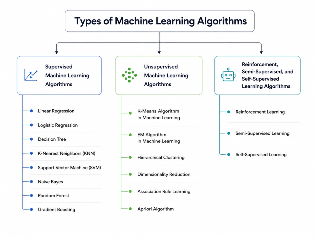
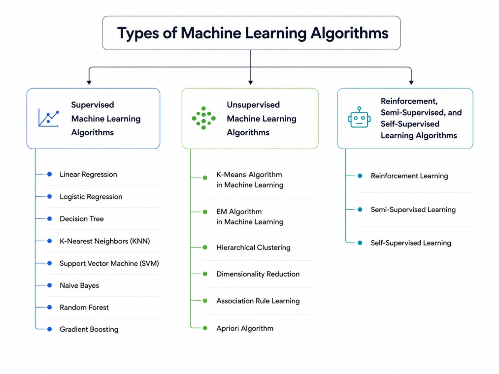
1. Supervised Machine Learning Algorithms
Supervised learning algorithms are trained on labeled data, meaning every input in the training set comes with a known, correct output. The algorithm's job is to learn the mapping between the two so it can predict outputs for new, unlabeled inputs.
They are mainly used for classification and regression problems.
1.1. Linear Regression
Linear regression is a type of supervised learning algorithm that is used to predict numerical values, such as house prices or salaries. This algorithm studies the relationship between input factors and the value you want to predict.
Best use cases involved:
House price prediction
Sales forecasting
Revenue estimation
Demand prediction
Advantages of Linear Regression:
Limitations of Linear Regression:
It performs poorly when relationships are highly complex
It is also sensitive to extreme values
It requires suitable feature relationships
Python example:
from sklearn.linear_model import LinearRegression
X = [[1], [2], [3], [4]]
y = [10, 20, 30, 40]
model = LinearRegression()
model.fit(X, y)
prediction = model.predict([[5]])
print(prediction)
Output: [50.]
1.2. Logistic Regression
Logistic Regression is one of the most commonly used machine learning classification algorithms. It predicts the probability of an input belonging to a particular category, such as whether an email is spam or not spam.
Best use cases:
Advantages:
Limitations:
Not suitable for highly complex relationships
Performance can suffer when classes are not well separated
Requires suitable feature representation
Python example:
from sklearn.linear_model import LogisticRegression
X = [[1], [2], [3], [4], [5], [6]]
y = [0, 0, 0, 1, 1, 1]
model = LogisticRegression()
model.fit(X, y)
prediction = model.predict([[5]])
print(prediction)
Output: [1]
1.3. Decision Tree
A Decision Tree is a machine learning algorithm that makes predictions by asking a series of simple questions about the data. It splits the data based on different features and follows a tree-like shape to reach a result.
For example, it can predict whether a customer will buy a product based on their age, income, and past purchases.
Best use cases:
Customer classification
Loan approval
Medical diagnosis
Risk assessment
Advantages:
Limitations:
Can overfit training data
Small changes in data can produce a different tree
Very deep trees can become difficult to generalise
Python example:
from sklearn.tree import DecisionTreeClassifier
X = [[1], [2], [3], [4], [5], [6]]
y = [0, 0, 0, 1, 1, 1]
model = DecisionTreeClassifier(random_state=42)
model.fit(X, y)
prediction = model.predict([[5]])
print(prediction)
Output: [1]
1.4. K-Nearest Neighbors (KNN)
The KNN algorithm in machine learning classifies a data point based on the labels of nearby observations. Instead of learning a complex mathematical representation during training, it compares a new observation with existing data points.
Best use cases:
Advantages:
Limitations:
Prediction can become slow with large datasets
Sensitive to feature scaling
Choosing an appropriate value of K can affect performance
Python example:
from sklearn.neighbors import KNeighborsClassifier
X = [[1], [2], [3], [6], [7], [8]]
y = [0, 0, 0, 1, 1, 1]
model = KNeighborsClassifier(n_neighbors=3)
model.fit(X, y)
prediction = model.predict([[5]])
print(prediction)
Output: [1]
1.5. Support Vector Machine (SVM)
Support Vector Machine creates a decision boundary that separates different classes. It aims to find a boundary that provides the best separation between groups.
Best use cases:
Advantages:
Effective for high-dimensional data
Can handle complex boundaries using kernels
Works well with smaller datasets in suitable cases
Limitations:
Can require significant computation for large datasets
Sensitive to feature scaling
Choosing the right kernel and parameters can be challenging
Python example:
from sklearn.svm import SVC
X = [[1], [2], [3], [6], [7], [8]]
y = [0, 0, 0, 1, 1, 1]
model = SVC()
model.fit(X, y)
prediction = model.predict([[5]])
print(prediction)
Output: [1]
1.6. Naive Bayes
Naive Bayes is a probabilistic classification algorithm based on Bayes' theorem. It assumes that features are conditionally independent given the class.
Best use cases:
Advantages:
Limitations:
The independence assumption may not always hold
Can perform poorly when features have strong dependencies
Probability estimates may require calibration in some applications
Python example:
from sklearn.naive_bayes import GaussianNB
X = [[1, 2], [2, 1], [8, 9], [9, 8]]
y = [0, 0, 1, 1]
model = GaussianNB()
model.fit(X, y)
prediction = model.predict([[7, 8]])
print(prediction)
Output: [1]
1.7. Random Forest
The Random Forest algorithm in machine learning combines multiple decision trees to produce a prediction. Each tree learns from a different sample of the data and feature combinations, and their outputs are combined.
Best use cases:
Advantages:
Limitations:
Python example:
from sklearn.ensemble import RandomForestClassifier
X = [[1], [2], [3], [6], [7], [8]]
y = [0, 0, 0, 1, 1, 1]
model = RandomForestClassifier(
n_estimators=100,
random_state=42
)
model.fit(X, y)
prediction = model.predict([[5]])
print(prediction)
Output: [1]
1.8. Gradient Boosting
Gradient Boosting builds models sequentially. Each new model focuses on reducing the errors made by the previous models.
Best use cases:
Advantages:
Can provide strong predictive performance
Handles different types of prediction problems
Can model complex relationships
Limitations:
Training can take longer than simpler algorithms
Sensitive to parameter settings
Excessive model complexity can cause overfitting
Python example:
from sklearn.ensemble import GradientBoostingClassifier
X = [[1], [2], [3], [6], [7], [8]]
y = [0, 0, 0, 1, 1, 1]
model = GradientBoostingClassifier(random_state=42)
model.fit(X, y)
prediction = model.predict([[5]])
print(prediction)
Output: [1]
2. Unsupervised Machine Learning Algorithms
Unsupervised machine learning algorithms work with data that does not have predefined labels or answers. They analyze the data to find hidden patterns, groups, and relationships on their own. For example, they can group customers with similar buying habits without being told which group each customer belongs to.
2.1. K Means Algorithm in Machine Learning
The K Means algorithm in machine learning groups data points into a predefined number of clusters. It assigns each observation to the nearest cluster centre and repeatedly updates the centres until the groups stabilise.
Best use cases:
Customer segmentation
Grouping products
Market analysis
Document clustering
Advantages:
Simple and easy to understand
Works well with large datasets
Fast for many clustering tasks
Limitations:
Python example:
from sklearn.cluster import KMeans
X = [[1, 2], [1, 3], [2, 2], [8, 8], [9, 8], [8, 9]]
model = KMeans(n_clusters=2, random_state=42, n_init=10)
model.fit(X)
print(model.labels_)
Output: [0 0 0 1 1 1]
2.2. EM Algorithm in Machine Learning
The EM algorithm in machine learning, or Expectation-Maximization algorithm, estimates unknown parameters when the data contains hidden or unobserved variables. It alternates between estimating the hidden assignments and updating the model parameters.
Best use cases:
Clustering
Missing-data problems
Statistical modelling
Mixture models
Advantages:
Useful when hidden variables are involved
Can work with incomplete datasets
Provides a flexible approach to probability-based modelling
Limitations:
Can converge to a local optimum
Results can depend on initial parameter values
May require several iterations to converge
Python example:
from sklearn.mixture import GaussianMixture
X = [[1, 2], [1, 3], [2, 2], [8, 8], [9, 8], [8, 9]]
model = GaussianMixture(n_components=2, random_state=42)
model.fit(X)
print(model.predict(X))
Output: [1 1 1 0 0 0]
2.3. Hierarchical Clustering
Hierarchical clustering creates a hierarchy of groups by progressively combining similar observations or dividing larger groups into smaller ones. The results can be represented through a dendrogram.
Best use cases:
Advantages:
Does not always require the number of clusters in advance
Produces a hierarchy of clusters
Useful for exploring relationships between observations
Limitations:
Computationally expensive for large datasets
Sensitive to the distance metric and linkage method
Early grouping decisions cannot easily be reversed
Python example:
from sklearn.cluster import AgglomerativeClustering
X = [[1, 2], [1, 3], [2, 2], [8, 8], [9, 8], [8, 9]]
model = AgglomerativeClustering(n_clusters=2)
labels = model.fit_predict(X)
print(labels)
Output: [1 1 1 0 0 0]
2.4. Dimensionality Reduction
Dimensionality reduction reduces the number of features in a dataset while retaining as much useful information as possible. It can make complex datasets easier to analyse and visualise.
Best use cases:
Advantages:
Reduces the number of features
Can improve processing speed
Helps visualise complex datasets
Limitations:
Some information may be lost
Reduced features can be harder to interpret
Results depend on the selected technique
Python example:
from sklearn.decomposition import PCA
X = [
[2, 4, 6],
[3, 6, 9],
[4, 8, 12],
[5, 10, 15]
]
model = PCA(n_components=2)
reduced_data = model.fit_transform(X)
print(reduced_data)
Output:
[[-5.61248608e+00 -1.40576383e-17]
[-1.87082869e+00 3.83390135e-18]
[ 1.87082869e+00 -3.83390135e-18]
[ 5.61248608e+00 -1.15017040e-17]]
2.5. Association Rule Learning
Association rule learning identifies relationships between items or events that frequently occur together. It is often used to discover patterns in transaction data.
Best use cases:
Advantages:
Finds relationships within large transaction datasets
Useful for recommendation systems
Easy to interpret when rules are simple
Limitations:
Can generate a large number of rules
Results depend on support and confidence thresholds
Strong associations do not necessarily indicate causation
Simple example:
transactions = [
{"bread", "milk"},
{"bread", "butter"},
{"bread", "milk", "butter"}
]
for transaction in transactions:
if "bread" in transaction and "milk" in transaction:
print("Bread and milk occur together")
This basic example checks whether two items occur together in transactions.
2.6. Apriori Algorithm
The Apriori algorithm identifies frequent item sets and uses them to generate association rules. It works by finding item combinations that meet a specified minimum support level.
Best use cases:
Advantages:
Limitations:
Can become slow with large datasets
Generates many candidate itemsets
Requires suitable support and confidence thresholds
Python example:
from mlxtend.frequent_patterns import apriori
import pandas as pd
data = pd.DataFrame({
"Bread": [1, 1, 1, 0],
"Milk": [1, 1, 0, 1],
"Butter": [0, 1, 1, 1]
})
frequent_items = apriori(
data,
min_support=0.5,
use_colnames=True
)
print(frequent_items)
Output:
support itemsets
0 0.75 (Bread)
1 0.75 (Milk)
2 0.75 (Butter)
3 0.50 (Bread, Milk)
4 0.50 (Bread, Butter)
5 0.50 (Milk, Butter)
Reinforcement, Semi-Supervised, and Self-Supervised Learning Algorithms
Not all machine learning tasks fit neatly into supervised or unsupervised learning. Some approaches learn through interaction, combine labelled and unlabelled data, or create learning signals directly from the available data.
Reinforcement Learning
Reinforcement learning trains an agent through interaction with an environment. The agent takes actions and receives rewards or penalties, gradually learning which actions lead to better outcomes.
Best use cases:
Robotics
Game-playing systems
Recommendation systems
Resource management
Advantages:
Learns through interaction
Works well for sequential decision-making
Can adapt its behaviour based on feedback
Limitations:
Can require large amounts of training
Designing suitable reward functions can be difficult
Training may be computationally expensive
Python example:
actions = ["left", "right", "stay"]
rewards = {"left": 0, "right": 1, "stay": -1}
best_action = max(actions, key=lambda action: rewards[action])
print(best_action)
Output: right
Semi-Supervised Learning
Semi-supervised learning combines a small amount of labelled data with a larger amount of unlabelled data. This approach is useful when obtaining labels for every observation is costly or time-consuming.
Best use cases:
Advantages:
Reduces the need for large labelled datasets
Makes use of available unlabelled data
Can improve learning when labelled data is limited
Limitations:
Incorrect assumptions about unlabelled data can affect results
Requires careful data preparation
Performance depends on the quality of both labelled and unlabelled data
Python example:
from sklearn.semi_supervised import LabelSpreading
X = [[1], [2], [3], [7], [8], [9]]
y = [0, 0, -1, 1, 1, -1]
model = LabelSpreading()
model.fit(X, y)
print(model.transduction_)
Output: [0 0 0 1 1 1]
Self-Supervised Learning
Self-supervised learning creates training signals from the data itself. Instead of requiring manually labelled examples, the system creates a learning task from the available information.
Best use cases:
Advantages:
Reduces dependence on manually labelled data
Can learn useful data representations
Suitable for large datasets
Limitations:
Designing effective pretext tasks can be challenging
Training can require substantial computing resources
Learned representations may not always suit every downstream task
Simple Python example:
text = "Machine learning algorithms learn from data"
words = text.split()
for i in range(len(words) - 1):
input_word = words[i]
target_word = words[i + 1]
print(input_word, "->", target_word)
Output: Machine -> learning learning -> algorithms algorithms -> learn learn -> from from -> data
When to Use Each Learning Approach
Learning Approach | Use When | Typical Applications |
Supervised Learning | You have labelled data and a known target | Classification, regression |
Unsupervised Learning | You want to discover hidden patterns | Clustering, dimensionality reduction |
Reinforcement Learning | An agent needs to learn through actions and rewards | Robotics, games, decision-making |
Semi-Supervised Learning | You have limited labelled data and plenty of unlabelled data | Image and text classification |
Self-Supervised Learning | You have large amounts of unlabelled data | NLP, computer vision, speech |
The best approach depends on the type of data available, the problem you want to solve, and how the model is expected to learn.
These are the types of ML algorithms that are used to train different types of Machine learning models. Now let’s see how these are used in different industries in real world applications.
Machine Learning Algorithms for Different Applications
Machine learning algorithms are only useful in the context of a real problem, and the right choice often depends on the industry. Let’s explore the applications of machine learning algorithms in different industries:
In healthcare, supervised algorithms like Random Forest and Gradient Boosting are used to predict disease risk and support diagnostic decisions, while clustering algorithms help group patients by similar symptoms or treatment responses.
In fraud detection, classification algorithms such as Logistic Regression, Random Forest, and anomaly-detection variants of clustering are trained on historical transaction data to flag suspicious activity in real time.
In e-commerce, association rule learning and KNN power recommendation engines, while classification algorithms predict customer churn and lifetime value.
In finance, regression algorithms forecast stock trends and credit risk, and reinforcement learning is increasingly used in algorithmic trading strategies.
In manufacturing, machine learning algorithms support predictive maintenance by classifying sensor readings as normal or likely-to-fail.
Now let’s see how to choose between all algorithms as it may confuse beginners due to a wide number of algorithms available.
How to Choose the Right Machine Learning Algorithm
There is no single best machine learning algorithm for every problem. The right choice depends on the nature of the problem and the data available.
Choose an Algorithm Based on the Problem
Start by identifying what kind of output you need. First, if you are predicting a category, you need machine learning classification algorithms. Second, if you are predicting a continuous number, you need a regression algorithm. Third, if you are grouping similar items with no predefined labels, you need a clustering algorithm. Sequential decision-making problems point toward reinforcement learning.
Choose an Algorithm Based on the Dataset
Your dataset can also influence which algorithm is appropriate for your needs.
Small datasets: KNN, Logistic Regression, SVM, and Decision Trees can be useful starting points.
Large datasets: K-Means, Random Forest, and Gradient Boosting can handle many practical large-scale tasks.
High-dimensional data: SVM and dimensionality reduction methods can be useful.
Unlabelled data: K-Means, Hierarchical Clustering, and EM are suitable options.
Labelled data: Supervised algorithms such as Linear Regression, Logistic Regression, Decision Trees, and Random Forest can be considered.
Key Factors for Algorithm Selection
Before choosing a machine learning algorithm, you have to evaluate these factors:
Dataset size: Large datasets may require algorithms that can process data efficiently.
Data type: Check whether your data is numerical, categorical, text-based, image-based, or mixed.
Target variable: Identify whether you need a numerical prediction, classification, or grouping.
Accuracy requirements: Some applications require highly accurate predictions, while others may prioritise simplicity.
Interpretability: Choosing an easier-to-understand model when explaining predictions is important.
Training time: Complex algorithms may require more time and computing resources.
Computational resources: Consider available CPU, memory, GPU, and storage capacity.
How to Improve Machine Learning Algorithm Performance
Selecting an algorithm is only one part of building a good model. You also need to prepare your data, control model complexity, tune parameters, and evaluate performance properly.
How to Handle Overfitting
Overfitting occurs when a model learns the training data too closely and performs poorly on unseen data. To fix overfitting, you need to help your machine learning model focus on general patterns instead of memorizing noise in your training data.
Key Fixes for Overfitting
Get more data: Use a larger and more varied dataset.
Use data augmentation: Create modified training examples, such as rotated images.
Simplify the model: Use fewer layers, neurons, or a simpler algorithm.
Apply regularization: Add a penalty to prevent the model from relying too much on specific features.
Use early stopping: Stop training when the model stops improving on new data.
How to Handle Underfitting
Underfitting occurs when a model is too simple to capture important patterns in the data.
You can address it by:
Using a more suitable algorithm
Adding relevant features
Increasing model complexity
Reducing excessive regularisation
Training the model for an appropriate number of iterations
How to Tune Machine Learning Algorithms
Hyperparameter tuning helps you find settings that produce better model performance.
Common approaches include:
Grid Search: Tests a defined combination of parameter values.
Random Search: Tests randomly selected parameter combinations.
Cross-Validation: Evaluates model performance across different portions of the dataset.
Bayesian Optimisation: Uses previous results to guide the search for better parameters.
Genetic Algorithms for Model Optimisation
Genetic algorithm machine learning uses an evolutionary approach to search for better solutions. In machine learning, it can help select features, tune hyperparameters, or identify suitable combinations of model settings.
The process generally involves:
Creating a population of possible solutions
Evaluating each solution
Selecting better-performing solutions
Applying crossover and mutation
Repeating the process for multiple generations
This Genetic algorithm machine learning approach can be useful when the search space is large and traditional parameter search methods are less suitable.
Common Mistakes When Choosing an Algorithm
Avoid these common mistakes when selecting a machine learning algorithm:
Choosing an algorithm only because it is popular
Ignoring the size and quality of your dataset
Using accuracy as the only performance measure
Selecting a complex model for a simple problem
Failing to separate training and testing data
Ignoring feature scaling when an algorithm requires it
Overlooking model interpretability
Tuning the model against the test dataset
Now let’s explore some of the problems and projects which you can do by yourself to get hands-on experience with machine learning algorithms.
Practice Problems and Projects to Learn Machine Learning Algorithms
Practical exercises help you understand when and why to use different algorithms. Start with simple datasets before moving to larger projects.
1. Classification Problem
Build a model that predicts whether a customer will leave a service based on factors such as usage, tenure, and account details.
Try: Logistic Regression, Decision Tree, Random Forest, or SVM.
2. Regression Problem
Create a model that predicts house prices using features such as size, location, number of rooms, and property age.
Try: Linear Regression or Gradient Boosting.
3. Clustering Problem
Group customers according to spending patterns, purchase frequency, or engagement.
Try: K-Means or Hierarchical Clustering.
4. Algorithm Selection Problem
Take the same dataset and test multiple algorithms. Compare their results using appropriate evaluation metrics.
For example:
Train Logistic Regression
Train Decision Tree
Train Random Forest
Compare their performance
Identify which model best fits the problem
Practical Projects to Learn Machine Learning Algorithms
You can build projects around real life problems such as:
Machine Learning Libraries for Implementing Algorithms
Python provides several libraries that make it easier to build and test machine learning models.
Scikit-learn: Common algorithms such as regression, classification, clustering, and dimensionality reduction.
Pandas: Data loading, cleaning, and manipulation.
NumPy: Numerical operations and array processing.
Matplotlib: Data visualisation.
XGBoost: Gradient boosting for classification and regression tasks.
Conclusion
Machine learning algorithms provide different approaches for learning patterns from data, making predictions, grouping observations, and solving decision-making problems. Supervised, unsupervised, reinforcement, semi-supervised, and self-supervised methods each serve different purposes.
To select the right algorithm, start with your problem and dataset. Then consider accuracy, interpretability, training time, data size, and available computing resources. Practicing with classification, regression, and clustering projects can help you understand how different algorithms perform in real-world situations.