Random Forest Algorithm in Machine Learning: Working, Types, Pseudocode

Quick Overview:

• The random forest is one of the most powerful ensemble ML algorithms that combines multiple decision trees to improve predictions and reduce overfitting.

• It is a supervised learning technique that is used for both classification (predicting a category) and regression tasks (predicting a continuous value).

• It uses bootstrap sampling and random feature selection to create diverse decision trees, then combines their predictions through majority voting.

• In this blog, you will learn about the Random Forest Algorithm in Machine Learning in detail, including its working, key concepts, pseudocode, and implementation using Python.

What Is Random Forest Algorithm?

The random forest algorithm is one of the most reliable and widely used algorithms in machine learning. It is a popular supervised machine learning technique used for both classification and regression tasks.

Instead of relying on a single decision tree, It combines multiple decision trees (hence the name “forest”) to produce more reliable predictions and reduce the risk of overfitting. 

Explaining what is random forest algorithm in simple words is like asking the same question to a group of experts and going with the majority, instead relying on a single expert. 

Each tree in a random forest algorithm in machine learning is trained on a slightly different version of the data and considers a different random subset of features at each split, which means individual trees end up making different mistakes. When their predictions are combined, those individual errors tend to cancel out, which is the core idea that makes random forest so effective. 

Random Forest vs Decision Tree

If you are confused with the difference between Random Forest and Decision Tree, the table below helps you to differentiate between both:

The working of random forest algorithm in machine learning helps you to understand the topic more clearly. So, now let’s explore how a random forest algorithm works.

How Does the Random Forest Algorithm Work?

The random forest algorithm in ML works through a five-step process that repeats across every tree in the forest, combining randomness at two separate stages, in the data used and the features considered, to keep individual trees different from one another. 

The algorithm follow these key steps:

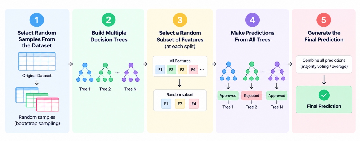
Step 1: Select Random Samples From the Dataset

Before training each individual tree, the random forest algorithm creates a new training set by randomly sampling rows from the original dataset with replacement, a technique called bootstrap sampling.

If the original dataset contains n rows, each bootstrap sample also has n rows, but because sampling happens with replacement, some original rows appear multiple times in a given bootstrap sample while others are left out entirely. 

Why sampling with replacement is used:  Sampling with replacement is what allows each tree to see a genuinely different version of the training data, even though every bootstrap sample is drawn from the same original dataset. This variation between samples is a key source of the diversity that makes combining many trees more powerful than relying on one. 

Step 2: Build Multiple Decision Trees

A separate decision tree is trained on each bootstrap sample. The trees are allowed to learn different relationships from their respective samples. Since each tree receives different training data and later considers random subsets of features, the resulting trees are not identical.

The forest can contain dozens, hundreds, or even thousands of trees, depending on the dataset and model configuration.

Step 3: Select a Random Subset of Features

At each split in a decision tree, the random forest considers only a randomly selected subset of available features instead of evaluating every feature. This is called feature randomness.

• For example, if a dataset has 20 features, a particular split might evaluate only a smaller subset of those features. Another tree or another split may consider a different subset.

Feature randomness reduces the correlation between trees, allowing the forest to benefit from having diverse individual models.

Step 4: Make Predictions From All Trees

After training, every decision tree produces its own prediction for a new observation.

For classification, the random forest generally uses majority voting. If most trees predict "Approved" and fewer trees predict "Rejected", the forest predicts "Approved".

For regression, the predictions from the individual trees are typically averaged to generate the final numerical prediction.

Step 5: Generate the Final Prediction

The final prediction combines the outputs of all individual trees.

• For classification: Final class = Class receiving the most votes

• For regression: Final prediction = Average of tree predictions

Combining many trees helps reduce the impact of errors made by individual trees. This is one reason the random forest can offer better generalization and lower variance than a single decision tree.

Let’s check out the key concepts, which are needed to understand the working of random forest algorithm.

Key Concepts Behind Random Forest

Few core concepts explain why the random forest algorithm works as well as it does, and understanding them makes the rest of the topic more understandable.

What Is Bagging?

Bagging, or Bootstrap Aggregating, is an ensemble learning technique that trains multiple models on different bootstrap samples of the same dataset and combines their predictions.

Random Forest uses bagging as one of its core ideas. However, it also introduces random feature selection, which helps create additional diversity among the trees.

How Does Bootstrap Sampling Work?

Bootstrap sampling creates a training sample by randomly selecting observations from the original dataset with replacement.

Suppose the original dataset contains: A, B, C, D, E

A bootstrap sample could be: A, C, C, E, B

Here, C appears twice while D does not appear. Another tree receives a different bootstrap sample. Repeating this process for many trees creates diverse training datasets.

What Is Feature Randomness?

Feature randomness refers to the practice of restricting each split within a tree to a randomly chosen subset of the available features, rather than allowing it to consider every feature in the dataset.

For example, a dataset may contain:

• Age

• Income

• Credit Score

• Employment Status

• Loan Amount

• Existing Debt

Instead of considering all six features at every split, the algorithm may consider only a randomly selected subset. This prevents individual trees from becoming too similar and strengthens the ensemble.

How Are Features Selected?

At each node, the algorithm selects a random subset of available features and evaluates potential splits using a chosen criterion.

• For classification, criteria such as Gini impurity or entropy can be used. 

• For regression, criteria based on prediction error, such as squared error, are commonly used.

The best split from the available feature subset is selected, and the tree continues growing recursively.

What Is Out-of-Bag Error?

Because bootstrap sampling uses replacement, some observations from the original dataset are not selected for a particular tree's training sample. These observations are called out-of-bag (OOB) samples for that tree.

The model can use these unused observations to estimate its performance without requiring a separate validation dataset. The resulting measure is known as the out-of-bag error. It provides a convenient estimate of generalisation performance during training.

Now let’s see random forest algorithm pseudocode​, before going into the implementation in Python.

Random Forest Algorithm Pseudocode

The pseudocode for random forest algorithm describes the major steps used to create multiple decision trees and combine their predictions.

Pseudocode for Random Forest Classification

Input:

    Training dataset D

    Number of trees T

    Number of features to consider at each split m

For each tree from 1 to T:

    1. Create a bootstrap sample Dᵢ from D.

    2. Start building a decision tree using Dᵢ.

    3. At each node:

        a. Randomly select m features.

        b. Find the best split among those features.

        c. Divide the data using the selected split.

    4. Continue splitting until the stopping condition is reached.

    5. Store the completed decision tree.

For a new observation:

    6. Get the prediction from every decision tree.

    7. Count the votes for each class.

    8. Select the class with the highest number of votes.

Output:

    Final classification

Pseudocode for Random Forest Regression

Input:

    Training dataset D

    Number of trees T

    Number of features to consider at each split m

For each tree from 1 to T:

    1. Create a bootstrap sample Dᵢ from D.

    2. Build a decision tree using Dᵢ.

    3. At each node:

        a. Randomly select m features.

        b. Find the best split.

        c. Divide the data.

    4. Continue until the stopping condition is reached.

    5. Store the completed tree.

For a new observation:

    6. Get a numerical prediction from every tree.

    7. Calculate the average of all tree predictions.

Output:

    Final regression prediction

This pseudocode for random forest algorithm implementations, whether for classification or regression, follows the exact same five-step process we discussed earlier in this blog: bootstrap sampling, tree training with feature randomness, and combining predictions through voting or averaging.

Now let’s explore how to implement this pseudocode for random forest algorithm​ through Python.

Random Forest Algorithm in Python

In this section you will explore, complete random forest algorithm example in Python using scikit-learn, covering both a classifier and a regressor. Follow the below steps to implement Random forest algorithm in Python:

1. Installing the Required Library

Scikit-learn. The random forest algorithm in Python is most commonly implemented using scikit-learn, which provides ready-to-use RandomForestClassifier and RandomForestRegressor classes. If it is not already installed, it can be added with:

pip install scikit-learn

2. Building a Random Forest Classifier

Import the model.

import numpy as np

import pandas as pd

from sklearn.model_selection import train_test_split, cross_val_score

from sklearn.ensemble import RandomForestClassifier

from sklearn.metrics import accuracy_score, precision_score, recall_score, f1_score

Load the dataset.

np.random.seed(42)

n = 300

income = np.round(np.random.uniform(20000, 120000, n))

credit_score = np.round(np.random.uniform(300, 850, n))

existing_loans = np.random.randint(0, 4, n)

score = (income / 120000) 0.5 + (credit_score / 850) 0.5 - existing_loans * 0.1

approved = ((score + np.random.normal(0, 0.08, n)) > 0.45).astype(int)

df = pd.DataFrame({

    "Income": income,

    "CreditScore": credit_score,

    "ExistingLoans": existing_loans,

    "Approved": approved

})

X = df[["Income", "CreditScore", "ExistingLoans"]]

y = df["Approved"]

This dataset of 300 loan applications mirrors the kind of structured, tabular data where random forest algorithms tend to perform particularly well.

Split training and testing data.

X_train, X_test, y_train, y_test = train_test_split(

    X, y, test_size=0.2, random_state=42, stratify=y

)

Train the model.

clf = RandomForestClassifier(

    n_estimators=200,

    max_depth=6,

    random_state=42,

    oob_score=True

)

clf.fit(X_train, y_train)

print("OOB score:", clf.oob_score_)

print("Feature importances:", dict(zip(X.columns, clf.feature_importances_)))

Setting n_estimators=200 builds a forest of 200 individual trees, and oob_score=True calculates the out-of-bag error estimate covered earlier, giving a built-in accuracy check without needing a separate validation set.

Make predictions.

y_pred = clf.predict(X_test)

3. Building a Random Forest Regressor

When to use regression. A random forest regressor is used when the target variable is continuous rather than categorical, such as predicting a house price, a delivery time, or a sales forecast, using the same underlying bagging and feature randomness principles as the classifier version.

Basic implementation.

from sklearn.ensemble import RandomForestRegressor

from sklearn.metrics import mean_squared_error

np.random.seed(7)

size = np.round(np.random.uniform(500, 3500, n))

bedrooms = np.random.randint(1, 5, n)

age = np.round(np.random.uniform(0, 30, n))

price = 20000 + size 120 + bedrooms 8000 - age * 500 + np.random.normal(0, 15000, n)

df_house = pd.DataFrame({"Size": size, "Bedrooms": bedrooms, "Age": age, "Price": price})

X_reg = df_house[["Size", "Bedrooms", "Age"]]

y_reg = df_house["Price"]

X_train_r, X_test_r, y_train_r, y_test_r = train_test_split(

    X_reg, y_reg, test_size=0.2, random_state=42

)

reg = RandomForestRegressor(n_estimators=200, max_depth=8, random_state=42)

reg.fit(X_train_r, y_train_r)

y_pred_r = reg.predict(X_test_r)

4. Evaluating a Random Forest Model

Accuracy, Precision, Recall, F1-score.

python

print("Accuracy:", accuracy_score(y_test, y_pred))

print("Precision:", precision_score(y_test, y_pred))

print("Recall:", recall_score(y_test, y_pred))

print("F1-score:", f1_score(y_test, y_pred))

Running this classifier example produces an accuracy of roughly 0.87, a precision of roughly 0.85, a recall of roughly 0.94, and an F1-score of roughly 0.89, with an out-of-bag score of roughly 0.83, all consistent with each other and indicating a well-generalising model.

Mean squared error / RMSE.

mse = mean_squared_error(y_test_r, y_pred_r)

rmse = np.sqrt(mse)

print("RMSE:", rmse)

In the regression example, this produces an RMSE of roughly 17,270, meaning the model's price predictions are typically off by around that amount, which is a reasonable margin given the scale and noise built into the sample housing data.

Cross-validation.

cv_scores = cross_val_score(clf, X, y, cv=5)

print("Cross-validation scores:", cv_scores)

print("Mean CV accuracy:", cv_scores.mean())

Cross-validation trains and evaluates the model across five different train-test splits of the data rather than just one, giving a more reliable estimate of how the random forest algorithm will perform on data it has not seen, and it is generally good practice to check this alongside a single train-test split evaluation.

After the implementation of random forest through Python, it is also necessary to look into where the algorithm is applied in the real world.  So let’s explore them.

Real-World Applications of Random Forest

The random forest algorithm is used across a wide range of industries, some common applications include: 

Advantages and Limitations of Random Forest

Like any machine learning algorithm, Random Forest has its own set of advantages and limitations. Let’s explore the key pros and cons of the Random Forest algorithm below.

Advantages of Random Forest

1. Reduces overfitting: Combining multiple trees generally makes the model less sensitive to the patterns learned by any single tree.

2. Works for classification and regression: Random forest can solve both categorical and numerical prediction problems.

3. Handles nonlinear relationships: It can capture complex relationships between input features and the target without requiring a linear relationship.

4. Works with many features: The algorithm can handle datasets containing a large number of input variables.

5. Provides feature importance: Random forest models can estimate how useful different features are for making predictions.

Limitations of Random Forest

1. Less interpretable than a single decision tree: Understanding hundreds of trees is considerably more difficult than interpreting one tree.

2. Can require more computational resources: Training and storing many trees can consume more memory and processing power.

3. Prediction can be slower: The model must obtain predictions from multiple trees before producing the final result.

4. Large forests can become resource-intensive: Increasing the number of trees can improve stability, but it can also increase training time and memory usage.

5. Not always the best choice for every dataset: Other algorithms may outperform random forest on particular datasets, especially when carefully tuned gradient-boosting methods are more suitable.

Conclusion

The Random Forest Algorithm combines multiple decision trees to create a robust machine learning model for classification and regression. By using bootstrap sampling and random feature selection, it creates diverse trees and combines their predictions to improve generalisation.

The algorithm is particularly useful for structured datasets where strong predictive performance and relatively limited preprocessing are important.