Support Vector Machine (SVM) in Machine Learning: Algorithm, Types, Kernels, and Examples

Quick Overview:

• Support Vector Machine (SVM) is a supervised machine learning algorithm used mainly for classification, while it can also handle regression through SVR.

• SVM finds an optimal hyperplane by maximising the margin between different classes, with support vectors determining the position of the decision boundary.

• Linear SVM, SVC, SVR, and kernel-based SVM are common types, with kernels such as linear, polynomial, RBF, and sigmoid helping handle different data patterns.

• In this blog you will learn Support Vector Machine in detail along with its foundational concepts, working, types and basic implementation using Python.

What Is Support Vector Machine in Machine Learning?

So, what is Support Vector Machine algorithm, exactly? A support vector machine or SVM is a supervised learning algorithm used especially for the classification, but it can also be used for the regression tasks. 

The core idea behind the support vector machine algorithm is to find the boundary called a hyperplane, which is best separated data points belonging to different classes, while maximising the distance between that boundary and the closest data points from each class. 

Understanding this through a support vector machine example or real life analogy, makes it easy to understand the topic. Let’s understand it through an analogy:

• Imagine two groups of cars driving on two sides of a road. You want to draw a line between them. 

• You could draw the line anywhere between the cars, but the best line is the one exactly in the middle, keeping the same distance from both groups. 

A support vector machine in machine learning does something similar, instead of drawing any line that separates two classes of data points, it looks for the one line, or in higher dimensions, the one flat surface, that keeps the widest possible buffer between itself and the nearest points of each class. 

Let’s understand the same with a help of support vector machine diagram below:

In this support vector machine diagram above it separates two groups of data:

• Class A: Blue circles on the left.

• Class B: Orange triangles on the right.

• Decision Boundary: The solid black line that separates the two classes.

• Margin: The space between the dashed lines around the decision boundary. SVM tries to make this margin as wide as possible.

• Support Vectors: The points closest to the decision boundary. These points are important because they determine the position of the boundary.

• Feature 1 and Feature 2: The two measurements used to represent each data point.

Now let’s take a look on some of the benefits and disadvantages of support vector machine algorithm:

 Benefits of Support Vector Machine

• It works well with high-dimensional datasets.

• It can create effective decision boundaries for classification.

• The kernel functions allow it to handle nonlinear relationships.

• It can be used for both classification and regression.

• The model focuses on the most informative observations near the decision boundary.

Limitations of Support Vector Machine

• The training can become computationally expensive for very large datasets.

• Choosing the appropriate kernel and hyperparameters can require experimentation.

• Support Vector Machine performance can be affected by feature scaling.

• The resulting model can be difficult to interpret compared with simpler models.

If you are confused about the Kernel and other features discussed in the above section, don't worry. We will discuss them in more detail in the upcoming section. Before that let’s explore some foundational concepts behind the support vector machine in machine learning.

Foundational Concepts Behind the Support Vector Machine Algorithm

Before understanding the working of the support vector machine algorithm, it is important to understand the foundational concepts such as the hyperplane, support vectors, and margin. 

These concepts explain how Support Vector Machine separates classes and determines the best decision boundary.

What Is Hyperplane in a Support Vector Machine?

A hyperplane in SVM is the decision surface that separates data points belonging to different classes. In a two-dimensional dataset with two features, the hyperplane is simply a straight line.

In three dimensions, it becomes a flat plane, and in datasets with more than three features, it becomes a hyperplane, a flat surface that exists in that higher-dimensional space but is harder to visualise directly. Mathematically, a hyperplane in SVM is defined by the support vector machine formula:

w . x + b = 0

Where w is a vector of weights, x represents the input features, and b is a bias term, similar in spirit to the intercept in linear regression.

What Are Support Vectors?

Support vectors are the specific data points from the training set that sit closest to the hyperplane, on either side of it. These points are the most important observations in the entire dataset from the algorithm's perspective, since they are literally what define the position and orientation of the optimal hyperplane. 

Every other point further away from the boundary could be removed from the training data without changing the model at all, which is why the algorithm is named after these support vectors rather than the dataset as a whole.

What Is the Margin?

The margin is the distance between the hyperplane and the nearest support vectors on either side. A support vector machine specifically tries to maximise this margin, since a wider margin generally corresponds to a more confident, more generalisable separation between classes, while a narrow margin suggests the boundary is more sensitive to small changes in the data.

How Does SVM Find the Best Hyperplane?

Finding the best hyperplane is framed as an optimisation problem: maximise the margin subject to the constraint that every training point is correctly classified, or, in the soft margin case covered later, correctly classified with only a limited, penalised amount of error. 

This is typically solved using quadratic programming, a class of mathematical optimisation techniques well suited to problems with a quadratic objective, maximising the margin, and linear constraints, correctly separating the classes.

What Is the Decision Boundary?

The decision boundary is the practical, usable output of a trained support vector machine algorithm: it is the hyperplane itself, used to classify new, unseen observations. Any new data point is classified based purely on which side of the decision boundary it falls on, calculated by plugging its feature values into the hyperplane equation w . x + b and checking whether the result is positive or negative.

How Does the Support Vector Machine Algorithm Work?

The Support Vector Machine in Machine Learning works by changing the classification problem into a geometric optimization problem. It finds the decision boundary that separates different classes while maximizing the gap, or margin, between them.

Below is the full working process of Support Vector Machine algorithm in detail:

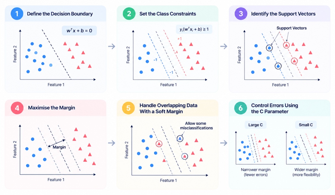
Step 1: Define the Decision Boundary

For a linearly separable dataset, SVM represents the decision boundary using a hyperplane. Its general equation is:

wᵀx + b = 0

Here, w is the weight vector perpendicular to the hyperplane, x represents the input features, and b is the bias term.

In two dimensions, this hyperplane appears as a straight line. With more features, it becomes a boundary in a higher-dimensional feature space.

Step 2: Set the Class Constraints

For binary classification, the support vector machine assigns the two classes the labels +1 and −1.

The model aims to position the hyperplane so that observations from the positive class fall on one side and observations from the negative class fall on the other. This can be expressed as:

yᵢ(wᵀxᵢ + b) ≥ 1

This constraint ensures that correctly classified observations are positioned on the appropriate side of the boundary.

Step 3: Identify the Support Vectors

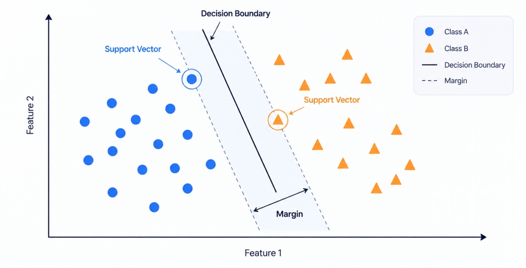
Once possible separating boundaries are considered, the support vector machine algorithm pays particular attention to the observations closest to the hyperplane. These are the support vectors.

Support vectors are important because they determine the position of the optimal boundary. Moving or removing these points can change the resulting hyperplane.

Step 4: Maximise the Margin

The margin represents the gap between the decision boundary and the closest observations from the two classes.

SVM aims to maximise this gap because a wider margin can provide better separation between classes. Mathematically, the margin is:

Margin = 2 / ||w||

Therefore, maximising the margin is equivalent to minimising the magnitude of the weight vector. The optimisation problem for a hard-margin support vector machine can be written as:

Minimise: ½||w||²

Subject to:

yᵢ(wᵀxᵢ + b) ≥ 1

The resulting hyperplane is the one that provides the maximum possible margin while satisfying the class constraints.

Step 5: Handle Overlapping Data With a Soft Margin

Real-world datasets are not always perfectly separable. Some observations may overlap or fall on the wrong side of the ideal boundary.

In such cases, support vector machine can use a soft margin, which allows controlled violations of the margin. Slack variables, represented by ξ (xi), quantify these violations.

This gives the model flexibility to handle noisy or overlapping data instead of forcing an unrealistic perfect separation.

Step 6: Control Errors Using the C Parameter

The C hyperparameter controls how strongly support vector machines penalize classification errors and margin violations.

• Large C: Places a higher penalty on errors, encouraging the model to classify training observations correctly. This can produce a narrower margin and may increase overfitting risk.

• Small C: Allows more margin violations in exchange for a wider margin, which can support better generalisation.

Thus, support vector machine in machine learning balances two objectives: creating a wide margin and limiting classification errors.

SVM can be used to solve different types of machine learning problems. Depending on the nature of the data and the task, SVMs can be implemented in different ways. Let us now look at the major types of Support Vector Machines.

Types of Support Vector Machines

Support Vector Machines can be categorised based on the prediction task and the type of decision boundary they use.

1. Support Vector Classification (SVC)

Support Vector Classification, or SVC, is the standard and most common form of support vector machine, used when the target variable is categorical. The algorithm finds a decision boundary that separates the classes while attempting to maximise the margin.

For example, an SVC model could classify:

• Spam vs non-spam

• Positive vs negative sentiment

• Fraudulent vs legitimate transaction

• Disease vs no disease

2. Support Vector Regression (SVR)

Support Vector Regression, or SVR, adapts the same core idea, maximising a margin around a boundary, to continuous target variables instead of categories. 

Rather than trying to keep data points as far as possible from a separating hyperplane, SVR tries to fit a function such that as many data points as possible fall within a specified margin, or tube, around that function, while still keeping the function as flat, or simple, as possible. 

3. Linear SVM

A linear SVM is used when the classes in the data can be separated reasonably well by a straight line, or a flat hyperplane in higher dimensions, without needing any additional transformation of the data. 

Linear SVM is computationally simpler and faster to train than kernel-based variants, and it is a sensible starting point whenever the underlying relationship between features and classes appears roughly linear.

4. Kernel-Based SVM

When a linear boundary cannot effectively separate the data, SVM can use kernel functions.

A support vector machine kernel allows the algorithm to work with nonlinear relationships by implicitly mapping the original data into a higher-dimensional feature space.

Common kernels include:

The RBF, or Radial Basis Function, kernel is commonly used when the relationship between features and classes is nonlinear.

Hard Margin vs Soft Margin Support Vector Machine

Support Vector Machine in Machine Learning can use either a hard-margin or soft-margin approach depending on whether classification errors are permitted.

What Is Hard Margin SVM?

Hard-margin SVM requires all training observations to be correctly classified and assumes that the classes can be completely separated by a hyperplane. It attempts to maximise the margin while allowing no classification violations.

However, real-world datasets often contain noise, outliers, or overlapping classes. In such cases, a hard margin may not be practical.

What Is Soft Margin SVM?

Soft-margin SVM allows some observations to violate the margin or even be classified incorrectly.

A penalty parameter, commonly represented by C, controls the trade-off between maximising the margin and penalising classification errors.

• Higher C: Places greater penalty on classification errors.

• Lower C: Allows more violations in exchange for a wider margin.

It is also important to view support vector machine algorithm in action. In the next section we will implement a support vector machine in Python using Scikit-learn.

How to Implement Support Vector Machine in Python

In this section you will find a complete support vector machine python example using scikit-learn, classifying two overlapping groups of data points, a support vector machine example chosen specifically to show how SVM handles classes that are not perfectly separable.

Import the Required Libraries

import numpy as np

import pandas as pd

import matplotlib.pyplot as plt

from sklearn.model_selection import train_test_split

from sklearn.preprocessing import StandardScaler

from sklearn.svm import SVC

from sklearn.metrics import accuracy_score, precision_score, recall_score, f1_score, confusion_matrix

Load and Explore the Dataset

np.random.seed(42)

n = 200

class0 = np.random.normal(loc=[3, 3], scale=1.6, size=(n // 2, 2))

class1 = np.random.normal(loc=[5.5, 5.5], scale=1.6, size=(n // 2, 2))

X = np.vstack([class0, class1])

y = np.array([0] (n // 2) + [1] (n // 2))

df = pd.DataFrame(X, columns=["Feature1", "Feature2"])

df["Label"] = y

print(df.head())

print(df["Label"].value_counts())

This creates two overlapping clusters of 100 points each, deliberately generated with enough spread that the classes are not perfectly separable, similar to how real-world classification data usually looks.

Prepare and Scale the Data

X_train, X_test, y_train, y_test = train_test_split(

    X, y, test_size=0.2, random_state=42, stratify=y

)

scaler = StandardScaler()

X_train_scaled = scaler.fit_transform(X_train)

X_test_scaled = scaler.transform(X_test)

Scaling the features before training matters more for SVM than for many other algorithms, since the algorithm's distance-based margin calculation is directly affected by the scale of each feature, and unscaled features can cause one variable to unfairly dominate the decision boundary.

Split the Dataset

The dataset was already split into training and test sets in the step above, keeping the class proportions balanced between both sets using stratify=y.

Train the SVM Model

model = SVC(kernel="rbf", C=1.0, gamma="scale")

model.fit(X_train_scaled, y_train)

print("Number of support vectors per class:", model.n_support_)

Here, kernel="rbf" selects the radial basis function kernel covered earlier, C=1.0 sets a moderate soft margin penalty, and gamma="scale" controls how far the influence of a single training example reaches, a parameter specific to the RBF kernel.

Make Predictions

y_pred = model.predict(X_test_scaled)

Evaluate the Model

python

print("Accuracy:", accuracy_score(y_test, y_pred))

print("Precision:", precision_score(y_test, y_pred))

print("Recall:", recall_score(y_test, y_pred))

print("F1-score:", f1_score(y_test, y_pred))

print("Confusion matrix:\n", confusion_matrix(y_test, y_pred))

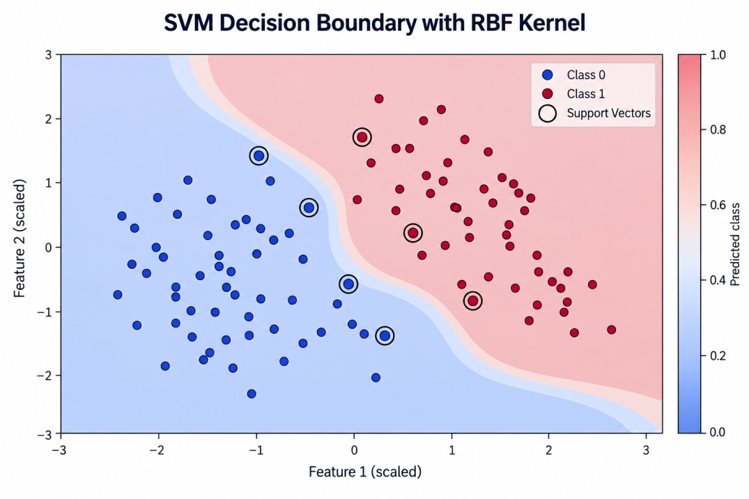
Running this example produces an accuracy of roughly 0.90, a precision of roughly 0.94, a recall of roughly 0.85, and an F1-score of roughly 0.89, with 28 and 27 support vectors identified for the two classes respectively. These numbers reflect exactly the kind of tradeoff a soft margin SVM is designed to make: since the two clusters genuinely overlap at their edges, a small number of misclassifications are accepted in exchange for a stable, generalisable decision boundary.

Visualise the Decision Boundary

xx, yy = np.meshgrid(

    np.linspace(X_train_scaled[:, 0].min() - 1, X_train_scaled[:, 0].max() + 1, 300),

    np.linspace(X_train_scaled[:, 1].min() - 1, X_train_scaled[:, 1].max() + 1, 300)

)

Z = model.predict(np.c_[xx.ravel(), yy.ravel()])

Z = Z.reshape(xx.shape)

plt.contourf(xx, yy, Z, alpha=0.2, cmap="coolwarm")

plt.scatter(

    X_train_scaled[:, 0], X_train_scaled[:, 1],

    c=y_train, cmap="coolwarm", edgecolors="k"

)

plt.scatter(

    model.support_vectors_[:, 0], model.support_vectors_[:, 1],

    s=100, facecolors="none", edgecolors="black", linewidths=1.5,

    label="Support Vectors"

)

plt.xlabel("Feature 1 (scaled)")

plt.ylabel("Feature 2 (scaled)")

plt.title("SVM Decision Boundary with RBF Kernel")

plt.legend()

plt.show()

Expected Output:

Now, let’s explore some real world applications of Support Vector Machine in Machine Learning.

Applications of Support Vector Machines

Support vector machines are used across different domains where classification or regression is required. Below are some common applications:

Conclusion

By now, we have understood that Support Vector Machine (SVM) is a powerful supervised learning algorithm that identifies an optimal decision boundary by maximizing the margin between classes. Concepts such as hyperplanes, support vectors, margins, kernels, and soft margins help us understand how SVM works and handles different types of data.

From classification and regression to nonlinear problems using kernel functions, SVM can be applied across several machine learning tasks. With proper feature scaling, kernel selection, and hyperparameter tuning, it can be an effective choice for many classification and regression problems.