Linear Regression in Machine Learning: Types, Algorithm, and Implementation

Quick Overview:

• Linear regression in machine learning predicts continuous numerical values by finding the best-fitting relationship between dependent and independent variables.

• It works by using an independent variable (X) to predict a dependent variable (Y), finding a best-fit line represented by Y = mX + b, and minimizing the difference between actual and predicted values.

• Simple, multiple, Ridge, and Lasso regression are the key types, for different datasets and modelling requirements.

• This blog covers linear regression in machine learning, types, applications, and Python code implementation with practical examples.

What Is Linear Regression in Machine Learning?

Linear Regression is one of the most widely used supervised machine learning algorithms which is used for predicting continuous numerical values. It is used to predict a continuous dependent variable from one or more independent variables.

Linear regression, models the relationship between dependent and independent variables by fitting a straight line to the observed data.

For understanding linear regression in machine learning in simple words, let’s understand it by an analogy-

Suppose you own an ice cream shop. You record the daily temperature and the number of ice creams you sell each day.

• When it is 20°C, you sell 70 cones.

• When it is 30°C, you sell 90 cones.

• When it is 50°C, you sell 150 cones.

Now, if you put these dots on a graph, you can use a ruler to draw a single straight line that passes as close to all the dots as possible. This line is your linear regression model in machine learning.

The next day the weather report says it will be 40°C. You look at your line on the graph at the 40°C mark, follow it up to the line, and see it predicts you will sell about 120 cones. That is linear regression in action.

Now let’s see how linear regression in machine learning works.

How Does Linear Regression Work?

Linear regression in machine learning works by finding the best-fitting line through the data. It does this by adjusting numbers called coefficients and a constant so that the predicted values are as close as possible to the actual values.

A linear regression algorithm generally follows these steps:

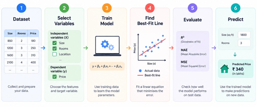
1. Collect a dataset containing input and target variables.

2. Identify the dependent and independent variables.

3. Fit a regression line to the training data.

4. Calculate the difference between actual and predicted values.

5. Minimise the prediction error using an optimization method.

6. Use the trained model to predict values for new data.

After exploring the basic working of linear regression in machine learning, the topic becomes now more clear. Now let’s explore the concepts and methods involved in working with linear regression model in machine learning.

1. Dependent and Independent Variables

Two main types of variables are used in Linear regression:

• Independent variable (X): The input or predictor used to make a prediction.

• Dependent variable (Y): The target value that the model aims to predict.

For example, if you are predicting house prices based on area:

• Independent variable = House area

• Dependent variable = House price

With multiple independent variables, the model could use area, number of bedrooms, location score, and property age to predict the price.

2. Linear Regression Equation

The linear regression in machine learning formula shows how the target variable is estimated from one or more input variables. For simple linear regression, the formula is:

y = β₀ + β₁x + ε

Where:

• y = predicted or dependent variable

• x = independent variable

• β₀ = intercept

• β₁ = regression coefficient or slope

• ε = error term

The equation for predictions, is commonly written as:

ŷ = β₀ + β₁x

Here, ŷ represents the predicted value.

For multiple linear regression in machine learning, the equation becomes:

ŷ = β₀ + β₁x₁ + β₂x₂ + ... + βₙxₙ

Each coefficient represents the expected change in the target variable when its corresponding input changes by one unit, assuming other variables remain constant.

3. How Is the Regression Line Calculated?

The regression line represents the relationship between the input and target variables. The algorithm searches for the line that provides the best fit to the available data.

Consider the equation:

ŷ = 10 + 2x

If x = 5, then:

ŷ = 10 + (2 × 5)

ŷ = 20

Therefore, the model predicts a value of 20.

The slope, 2, means that the predicted target increases by 2 units for every one-unit increase in x.

4. Least Squares Method in Linear Regression

The least squares method is commonly used to determine the best-fitting regression line. It minimises the sum of the squared differences between actual and predicted values.

The residual for each observation is:

Residual = Actual Value − Predicted Value

The sum of squared errors can be represented as:

SSE = Σ(yᵢ − ŷᵢ)²

The algorithm selects the coefficients that minimise this value. Squaring the errors prevents positive and negative errors from cancelling each other and gives greater weight to larger errors.

5. Cost Function in Linear Regression

A cost function measures how accurately the linear regression model predicts the target variable.

One commonly used cost function is Mean Squared Error (MSE):

MSE = (1/n) Σ(yᵢ − ŷᵢ)²

Where:

• n = number of observations

• yᵢ = actual value

• ŷᵢ = predicted value

A lower MSE indicates that predictions are, on average, closer to the actual values.

6. Gradient Descent in Linear Regression

Gradient descent is an optimisation technique that can be used to minimise the cost function.

The algorithm starts with initial values for the model parameters and repeatedly updates them in the direction that reduces the error.

The general update rule is:

θ = θ − α∇J(θ)

Where:

• θ = model parameters

• α = learning rate

• ∇J(θ) = gradient of the cost function

A suitable learning rate helps the algorithm converge efficiently. A very small learning rate can make training slow, while a very large learning rate can cause the optimization process to overshoot the minimum.

Linear regression can be used in different ways depending on the data and the number of input variables. So now, let’s explore the different types of linear regression in machine learning.

Types of Linear Regression in Machine Learning

Linear regression can be classified based on the number of predictors and whether regularization is applied. Below are main the types of linear regression:

1. Simple Linear Regression in Machine Learning

Simple linear regression in machine learning is a method in which a dependent variable is predicted using a single independent variable by fitting a straight line to the data.

Its equation is:

y = β₀ + β₁x + ε

For example, a company could predict monthly sales based only on its advertising expenditure.

Suppose:

Sales = 50 + 4 × Advertising Spend

If advertising spend is 10 units:

Sales = 50 + (4 × 10) = 90

The model therefore predicts sales of 90 units.

Simple linear regression in machine learning is easy to understand and visualize because it involves one predictor and one target variable.

2. Multiple Linear Regression in Machine Learning

Multiple linear regression in machine learning is a method in which a continuous target is predicted using two or more independent variables.

Its equation is:

y = β₀ + β₁x₁ + β₂x₂ + ... + βₙxₙ + ε

For example, house prices could be predicted using:

• House area

• Number of bedrooms

• Property age

• Distance from the city centre

A multiple regression in machine learning allows several factors to be considered at the same time. However, adding more variables does not always improve the model. Irrelevant or highly correlated variables can increase complexity and reduce model performance.

3. Regularised Linear Regression

Regularisation is a technique in which a penalty is added to the model’s objective function to limit large coefficients. It can help reduce overfitting, especially when a dataset contains many features.

Two common regularised approaches are Ridge and Lasso regression.

(a) Ridge Regression

Ridge regression is a method in which coefficients are generally reduced toward zero without being set exactly to zero. It can be useful when several predictors contribute to the target and multicollinearity is present.

A simplified objective function is:

MSE + λΣβⱼ²

Where λ controls the strength of regularisation.

(b) Lasso Regression

Lasso regression is a method in which some coefficients can be reduced to exactly zero, allowing the model to perform feature selection.

MSE + λΣ|βⱼ|

Ridge and Lasso are useful when a standard linear regression model is at risk of overfitting.

How to Perform Linear Regression in Machine Learning?

Performing linear regression in machine learning generally follows the same five-step workflow, regardless of which tool or programming language you use.

1. Define the Problem and Select Variables

First, identify the dependent variable you want to predict and the independent variable(s) that may influence it. Then, check whether a linear relationship is suitable for the data, as a straight-line model may give poor predictions for clearly non-linear relationships.

For example:

• Problem: Predict house prices.

• Target variable: House price

• Features: Area, bedrooms, location score, and property age

The quality and relevance of the selected features can strongly influence the final model.

2. Prepare and Split the Dataset

Before training, clean the dataset and handle missing values, duplicate records, and incorrect entries.

The dataset is usually divided into:

• Training data: Used to learn the model.

• Test data: Used to evaluate its performance on unseen observations.

A common approach is an 80:20 or 70:30 train-test split, although the appropriate split depends on the dataset.

3. Train the Linear Regression Model

Train the model using the training data. The algorithm calculates the coefficients that best fit the data by minimising the cost function using methods such as least squares or gradient descent. This is the stage where the model learns the relationship between the input variables and the target.

4. Evaluate the Model

After training, generate predictions using the test data and evaluate them using appropriate regression metrics such as:

• R-squared

• Mean Squared Error

• Mean Absolute Error

Do not confuse what these metrics means, as we will discuss all these metrics in the next section below.

5. Interpret the Results

Review the model’s coefficients to understand the relationship between the input variables and the target. A positive coefficient increases the prediction, while a negative coefficient decreases it. The coefficient size shows the strength of the effect when the variables are on similar scales.

These are the five basic steps which you will need to perform while training your model by linear regression in machine learning. Now let’s see how to evaluate any machine learning linear regression model.

How to Evaluate a Linear Regression Model?

To understand how accurately a linear regression model in machine learning​ performs on unseen data, there are some metrics which can be used. You can evaluate your model by using metrics such as: 

1. R-Squared

To measure how much of the variation in the dependent variable is explained by the model you can use R-squared (R²).

It can be expressed as:

R² = 1 − (SSres / SStot)

Where:

• SSres = Sum of squared residuals

• SStot = Total sum of squares

An R² value closer to 1 generally means that the model explains more of the variation in the target. However, a high R² does not always mean that the model is suitable or will perform well on new data.

2. Mean Squared Error

To calculate the average squared difference between actual and predicted values you can use Mean Squared Error. 

MSE = (1/n) Σ(yᵢ − ŷᵢ)²

MAE is expressed in the same unit as the dependent variable, which makes it easier to interpret directly. For example, an MAE of 5,000 on a salary prediction model means the model's predictions are, on average, off by 5,000 currency units. MAE is also less sensitive to outliers than MSE, since it does not square the errors.

3. Mean Absolute Error

To measure the average absolute difference between actual and predicted values you can Mean Absolute Error. 

MAE = (1/n) Σ|yᵢ − ŷᵢ|

For example, if the prediction errors are 2, 3, and 5:

MAE = (2 + 3 + 5) / 3 = 3.33

MAE is easy to interpret because it shows the average prediction error in the same units as the target variable.

How to Interpret Linear Regression Results

When interpreting a regression model, consider:

• Intercept: Expected target value when all predictors are zero.

• Coefficient: Expected change in the target for a one-unit change in a predictor, holding other variables constant.

• R²: Proportion of target variation explained by the model.

• MAE/MSE: Magnitude of prediction errors.

• Residuals: Differences between actual and predicted values.

A coefficient's statistical significance may also be examined when using statistical regression analysis.

Assumptions of Linear Regression in Machine Learning

Before applying linear regression in machine learning, it is important to check whether the data meets certain conditions. These conditions help ensure that the model produces reliable and meaningful results.

1. Linearity

Linearity assumes that a straight-line relationship is present between the independent and dependent variables. If the relationship is curved, accurate predictions may not be produced by a linear model. A scatter plot can be used to check this assumption.

2. Independence of Observations

Independence of observations means that each data point is unrelated to the others. If one observation influences another, the results may be misleading. This assumption is often violated in time series data, where values are related to previous observations.

3. Homoscedasticity

Homoscedasticity means that the variance of the residuals remains roughly constant across all levels of the independent variable. If the variance changes, heteroscedasticity occurs, which may appear as a funnel or cone shape in a residual plot.

4. Normality of Residuals

Normality of residuals means that the model’s errors are approximately normally distributed. This assumption is mainly important for reliable confidence intervals and hypothesis tests. A histogram or Q-Q plot can be used to check it.

5. Absence of Multicollinearity

Absence of multicollinearity means that the independent variables are not strongly correlated with each other. High correlation between variables can make the model’s coefficients unstable and difficult to interpret. VIF is commonly used to detect multicollinearity.

Linear Regression Implementation in Python

In this section you will go through a full linear regression in machine learning python code example and a linear regression in machine learning python implementation, using scikit-learn, one of the most widely used Python libraries for machine learning. 

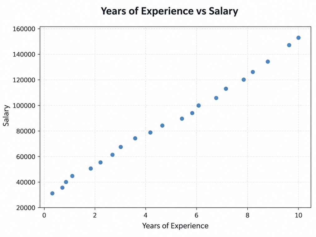
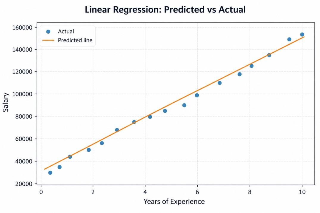
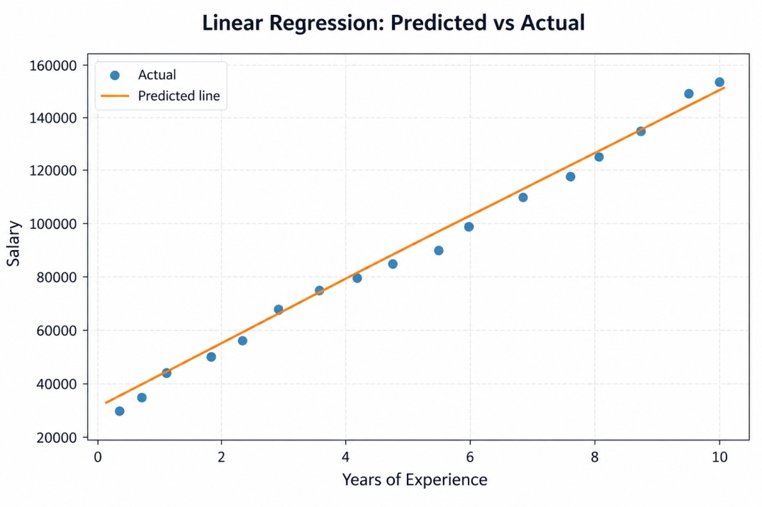
The example predicts salary from years of experience, a classic simple linear regression in machine learning example.

Import the Required Python Libraries

import numpy as np

import pandas as pd

import matplotlib.pyplot as plt

from sklearn.model_selection import train_test_split

from sklearn.linear_model import LinearRegression

from sklearn.metrics import mean_squared_error, mean_absolute_error, r2_score

Load and Explore the Dataset

np.random.seed(42)

years_experience = np.round(np.random.uniform(0, 12, 60), 1)

salary = 35000 + years_experience * 9500 + np.random.normal(0, 8000, 60)

df = pd.DataFrame({

    "YearsExperience": years_experience,

    "Salary": salary

})

print(df.head())

print(df.describe())

This creates a sample dataset of 60 employees with their years of experience and salary, with a realistic amount of random noise added so the relationship is linear but not perfectly clean, similar to real-world data.

Visualize the Variables

plt.scatter(df["YearsExperience"], df["Salary"], color="steelblue")

plt.xlabel("Years of Experience")

plt.ylabel("Salary")

plt.title("Years of Experience vs Salary")

plt.show()

Expected Output:

Prepare the Training and Test Data

X = df[["YearsExperience"]]

y = df["Salary"]

X_train, X_test, y_train, y_test = train_test_split(

    X, y, test_size=0.2, random_state=42

)

Train the Linear Regression Model

model = LinearRegression()

model.fit(X_train, y_train)

print("Intercept:", model.intercept_)

print("Coefficient:", model.coef_)

Running this code produces an intercept of roughly 37,017 and a coefficient of roughly 9,153 for years of experience. In other words, the model predicts a starting salary of about 37,017 for zero years of experience, with each additional year of experience adding approximately 9,153 to the predicted salary.

Make Predictions

y_pred = model.predict(X_test)

Evaluate the Model

mse = mean_squared_error(y_test, y_pred)

mae = mean_absolute_error(y_test, y_pred)

r2 = r2_score(y_test, y_pred)

print("MSE:", mse)

print("MAE:", mae)

print("R2:", r2)

On this sample dataset, the model achieves an R-squared of roughly 0.96, meaning it explains about 96 percent of the variance in salary based on years of experience alone, with an MAE of around 4,670, meaning predictions are off by about that amount on average.

Visualise the Regression Line

plt.scatter(X_test, y_test, color="steelblue", label="Actual")

plt.plot(X_test, y_pred, color="darkorange", linewidth=2, label="Predicted line")

plt.xlabel("Years of Experience")

plt.ylabel("Salary")

plt.title("Linear Regression: Predicted vs Actual")

plt.legend()

plt.show()

Expected Output:

Interpret the Coefficients

The trained model's coefficient of approximately 9,153 is the key business takeaway: for every additional year of experience in this dataset, predicted salary increases by about 9,153 units, holding nothing else constant since this is a simple linear regression in machine learning with only one input variable. 

This is the same interpretation logic that applies to multiple linear regression in machine learning, except each coefficient there represents the effect of its variable while holding all the other variables fixed, as shown in the multiple linear regression example below.

from sklearn.linear_model import LinearRegression

import numpy as np

import pandas as pd

np.random.seed(1)

n = 50

size_sqft = np.round(np.random.uniform(500, 3500, n))

bedrooms = np.random.randint(1, 5, n)

age_years = np.round(np.random.uniform(0, 30, n))

price = 20000 + size_sqft 120 + bedrooms 8000 - age_years * 500 + np.random.normal(0, 15000, n)

df_house = pd.DataFrame({

"Size_sqft": size_sqft,

"Bedrooms": bedrooms,

"Age_years": age_years,

"Price": price

})

X_multi = df_house[["Size_sqft", "Bedrooms", "Age_years"]]

y_multi = df_house["Price"]

multi_model = LinearRegression()

multi_model.fit(X_multi, y_multi)

print("Intercept:", multi_model.intercept_)

print("Coefficients:", dict(zip(X_multi.columns, multi_model.coef_)))

Expected Output: 

Intercept: 33488.48871651714

Coefficients: {

    'Size_sqft': 116.3513759283638,

    'Bedrooms': 8130.728223735531,

    'Age_years': -719.7535614838536

}

This multiple linear regression model in machine learning learns a separate coefficient for square footage, bedrooms, and property age, letting you see the individual contribution of each factor to the predicted house price.

Applications of Linear Regression in Machine Learning

Linear regression in machine learning is useful when the objective is to estimate a continuous numerical outcome.

Common applications include:

• House price prediction: Estimate property prices using area, location, rooms, and other features.

• Sales forecasting: Predict sales based on advertising expenditure, historical trends, or other business variables.

• Demand forecasting: Estimate product demand using historical and market data.

• Financial analysis: Model relationships between financial variables and estimate numerical outcomes.

• Healthcare: Estimate metrics such as treatment-related measurements or healthcare costs.

• Energy consumption: Predict electricity or energy usage based on relevant factors.

• Business analytics: Identify relationships between business inputs and measurable outcomes.

The suitability of a linear regression model in machine learning depends on whether the underlying relationship is sufficiently linear and whether the model's assumptions are reasonably satisfied.

Advantages and Limitations of Linear Regression

Like any algorithm, linear regression in machine learning is a strong fit for some problems and a poor fit for others, so it helps to weigh its advantages against its limitations before choosing it for a given dataset.

Advantages of Linear Regression

Linear regression remains popular because it is relatively simple and interpretable.

Its key advantages include:

• Easy to understand and implement

• Fast to train

• Computationally efficient

• Highly interpretable coefficients

• Works well as a baseline model

• Suitable for continuous target variables

• Supports statistical analysis and inference

• Can be extended using regularization

Limitations of Linear Regression

Despite its simplicity, linear regression has limitations:

• Assumes a linear relationship

• Can be sensitive to outliers

• Multicollinearity can affect coefficient interpretation

• May underperform on highly non-linear datasets

• Feature engineering may be required for complex relationships

• Basic models can be affected by irrelevant features

• High training performance does not guarantee good generalization

Conclusion

Linear regression in machine learning is a simple and interpretable approach for predicting continuous outcomes. It helps learners understand relationships between variables through regression equations, coefficients, and best-fit lines.

By understanding its types, assumptions, evaluation metrics, Python implementation, and common challenges, you can build more reliable models and identify situations where alternative machine learning algorithms may perform better.