Key Components of Reinforcement Learning
Every reinforcement learning problem is built from the same important components, and getting familiar will make the topic easier to understand. The key components of reinforcement learning in artificial intelligence are:
Component | Meaning |
Agent | The learner or decision-maker that interacts with the environment |
Environment | The world or system in which the agent operates |
State | The current situation of the agent |
Action | A decision or move the agent can make |
Reward | Feedback received after taking an action |
Policy | A strategy that determines which action to take in a given state |
Value Function | Estimates how valuable a state or action is based on expected future rewards |
Let’s take a reinforcement learning example to understand the components.
For example, in a self-driving car simulation, the car acts as the agent, the road and traffic form the environment, its current position represents the state, steering or braking are actions, and safe driving can generate positive rewards.
Also Read: Supervised vs Unsupervised Learning: Differences, Examples, and Applications
How Does Reinforcement Learning Work?
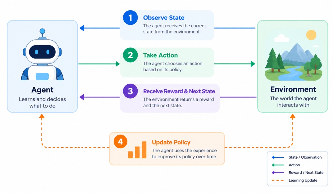
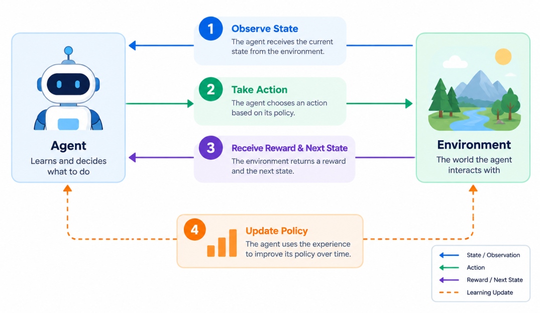
Reinforcement learning in machine learning works through a continuous feedback loop. The key steps it follows are:
The agent observes the current state of the environment.
It selects an action based on its current policy.
The environment responds to the action.
The agent receives a reward or penalty.
The environment moves to a new state.
The agent updates its knowledge based on the outcome.
This process continues until the agent learns a better policy.
The agent generally balances two behaviours:
The balance between exploration and exploitation is important because an agent that only exploits known actions may miss better strategies, while excessive exploration can slow learning.
As of now, the basics of reinforcement learning in AI are clear to you. Now let's see the Markov Decision Process (MDP), a mathematical framework commonly used to represent reinforcement learning problems.
Also Read: Logistic Regression in Machine Learning: Algorithm, Types, Examples, and Applications
Markov Decision Process in Reinforcement Learning
A Markov Decision Process in, or MDP in reinforcement learning in machine learning, is the formal mathematical framework used to describe reinforcement learning problems. Almost every reinforcement learning algorithms assumes the problem it is solving can be expressed as an MDP, which makes it worth understanding even at a high level.
An MDP is defined by five elements, usually written as a tuple:
MDP = (S, A, P, R, γ)
Where:
S = Set of possible states
A = Set of possible actions
P = Probability of transitioning from one state to another after an action
R = Reward received for an action
γ = Discount factor that determines the importance of future rewards
Example of an MDP
Consider a robot navigating a warehouse.
State: Robot's current location
Actions: Move forward, backward, left, or right
Transition: The robot moves to another location based on its action
Reward: Positive reward for reaching the destination and negative reward for hitting an obstacle
Policy: Strategy used by the robot to choose its next movement
The goal is to learn a policy that enables the robot to reach its destination while maximizing its total reward.
Now let's explore the major types of reinforcement learning and how they differ in the way an agent learns and makes decisions.
Advance your leadership journey with the Executive Programme in Technology & AI Leadership. Develop strategic technology and AI leadership skills to drive innovation, make informed decisions, and lead digital transformation.
Types of Reinforcement Learning in AI
Reinforcement learning approaches are commonly divided along two independent lines: whether the agent builds a model of its environment, and whether it learns values or learns a policy directly.
1. Model-Based Reinforcement Learning
Model-based reinforcement learning in machine learning uses a model of the environment to predict what may happen after an action. The agent attempts to understand the environment's transition dynamics and rewards. It can then use these predictions to plan future actions.
For example, a robot could learn that moving in a particular direction is likely to lead to a specific location and use this information to plan its route.
Key characteristics:
It uses an environment model.
It supports planning before taking actions.
It can be more data-efficient in some settings.
It requires learning or knowing the environment model.
2. Model-Free Reinforcement Learning
Model-free reinforcement learning in artificial intelligence does not explicitly build a model of the environment. Instead, the agent learns directly from its interactions and experiences. Algorithms such as Q-learning and many policy-gradient methods follow this approach.
The agent gradually learns which actions tend to produce better rewards without explicitly predicting every possible state transition.
Key characteristics:
It does not require an explicit environment model.
It learns directly from experience.
It may often be simpler to apply to complex environments.
It may require substantial interaction data.
Also Read: Decision Tree Algorithm in Machine Learning: How It Works, Types, and Examples
3. Value-Based Learning
Value-based reinforcement learning in AI focuses on estimating the value of states or actions. The agent learns how beneficial a particular state or action is in terms of expected future rewards. It then selects actions with higher estimated values.
Q-learning is a well-known example of a value-based reinforcement learning algorithm.
A commonly used Q-value update is:
Q(s, a) ← Q(s, a) + α[r + γ max Q(s', a') − Q(s, a)]
Where:
Also Read: Random Forest Algorithm in Machine Learning: Working, Types, Pseudocode
4. Policy-Based Learning
Policy-based reinforcement learning in machine learning directly learns a policy that determines which action an agent should take in a particular state.
Instead of first estimating the value of every action, the algorithm learns a strategy for selecting actions.
Policy-gradient methods are common examples of this approach. They can be particularly useful for problems with continuous action spaces, where an agent may need to choose from a large range of possible actions.
Now let's explore some of the major reinforcement learning algorithms and understand how they help agents learn effective decision-making strategies.
Major Reinforcement Learning Algorithms
A range of reinforcement learning algorithms have been developed, which differs mainly in how they estimate value, how they update their policy, and whether they use neural networks to handle complex state spaces.
Algorithm | Type | How It Works | Best Suited For |
Q-Learning | Model-free, value-based, off-policy | Learns a Q-value for each state-action pair using the Bellman equation, updating toward the best available next action | Discrete state and action spaces, foundational learning |
SARSA | Model-free, value-based, on-policy | Similar to Q-learning, but updates using the action the policy actually took rather than the best possible one | Situations where safer, more conservative learning matters |
Deep Q-Network (DQN) | Model-free, value-based, deep RL | Replaces the Q-table with a neural network, allowing it to handle very large or continuous state spaces | Complex visual environments, such as Atari games |
REINFORCE | Model-free, policy-based | Adjusts policy parameters directly in the direction that increases expected reward, using gradient ascent | Continuous action spaces, stochastic policies |
Actor-Critic | Model-free, hybrid | Combines a policy network (actor) with a value network (critic) that evaluates the actor's choices | Balancing the stability of value methods with policy flexibility |
PPO (Proximal Policy Optimisation) | Model-free, policy-based | Constrains how far the policy can change in a single update, improving training stability | Large-scale applications, including training language models |
Monte Carlo Methods | Model-free, value-based | Learns from complete episodes, updating value estimates using actual total returns rather than step-by-step estimates | Episodic tasks with clear endpoints |
Now let's explore how to actually implement one of these algorithms in code.
Also Read: Gradient Boosting Algorithm in Machine Learning: How It Works, and Practical Examples
How to Implement Reinforcement Learning in Python
In this section you will implement complete reinforcement learning example in Python, along with implementing Q-learning from scratch to train an agent to navigate a grid world.
1. Set Up the Environment
import numpy as np
np.random.seed(42)
GRID = 5
n_states = GRID * GRID
actions = ["up", "down", "left", "right"]
n_actions = len(actions)
GOAL = 24 # bottom-right corner
OBSTACLES = [7, 12, 17] # cells that penalise the agent
The environment is a 5x5 grid with 25 possible states. The agent starts in the top-left corner (state 0) and needs to reach the bottom-right corner (state 24), while avoiding three obstacle cells along the way.
2. Define the Agent
Q = np.zeros((n_states, n_actions))
alpha = 0.1 # learning rate
gamma = 0.9 # discount factor
epsilon = 1.0 # exploration rate, starts fully exploratory
eps_decay = 0.995
eps_min = 0.01
The agent is represented entirely by its Q-table, a grid of 25 states by 4 actions holding the estimated value of taking each action in each state. It starts filled with zeros, meaning the agent knows nothing at all. The epsilon value controls the exploration versus exploitation balance discussed earlier, starting at 1.0, meaning fully random exploration, and decaying gradually toward 0.01 as the agent gains experience.
3. Define States, Actions, and Rewards
def step(state, action_idx):
row, col = divmod(state, GRID)
if actions[action_idx] == "up":
row = max(row - 1, 0)
elif actions[action_idx] == "down":
row = min(row + 1, GRID - 1)
elif actions[action_idx] == "left":
col = max(col - 1, 0)
elif actions[action_idx] == "right":
col = min(col + 1, GRID - 1)
new_state = row * GRID + col
if new_state in OBSTACLES:
return state, -10, False # blocked, penalised, stays put
if new_state == GOAL:
return new_state, 100, True # reached the goal
return new_state, -1, False # ordinary step, small time penalty
The reward structure here does real work in shaping behaviour. Reaching the goal gives a large positive reward of 100, hitting an obstacle gives a penalty of -10, and every ordinary step gives a small penalty of -1. That small step penalty is what pushes the agent toward finding a short path rather than merely any path.
4. Choose a Reinforcement Learning Algorithm
This implementation uses Q-learning, the model-free, value-based algorithm from the table above. Its update rule is a direct application of the Bellman equation:
Q(s, a) = Q(s, a) + alpha [ reward + gamma max Q(s', a') - Q(s, a) ]
The term in brackets is the temporal difference error: the gap between what the agent expected the action to be worth and what it now estimates it is worth after seeing the actual reward and the value of the resulting state.
5. Train the Agent
episodes = 1000
rewards_log = []
for ep in range(episodes):
state = 0
total_reward = 0
for _ in range(100): # step limit per episode
# Epsilon-greedy action selection
if np.random.rand() < epsilon:
action = np.random.randint(n_actions) # explore
else:
action = np.argmax(Q[state]) # exploit
next_state, reward, done = step(state, action)
# Q-learning update
Q[state, action] = Q[state, action] + alpha * (
reward + gamma * np.max(Q[next_state]) - Q[state, action]
)
state = next_state
total_reward += reward
if done:
break
epsilon = max(eps_min, epsilon * eps_decay)
rewards_log.append(total_reward)
print("Average reward, first 100 episodes:", np.mean(rewards_log[:100]))
print("Average reward, last 100 episodes:", np.mean(rewards_log[-100:]))
Running this training loop produces an average reward of roughly 23.7 across the first 100 episodes and roughly 92.8 across the last 100, a clear demonstration that the agent genuinely learned from experience rather than continuing to wander randomly.
6. Evaluate the Learned Policy
state = 0
path = [state]
total_reward = 0
for _ in range(50):
action = np.argmax(Q[state]) # pure exploitation, no exploration
state, reward, done = step(state, action)
path.append(state)
total_reward += reward
if done:
break
print("Learned path:", path)
print("Steps taken:", len(path) - 1)
print("Total reward:", total_reward)
Evaluating the trained agent with pure exploitation produces the path [0, 5, 10, 15, 20, 21, 22, 23, 24], reaching the goal in 8 steps with a total reward of 93.
That 8-step route is genuinely optimal for this grid: moving from the top-left to the bottom-right of a 5x5 grid requires a minimum of 4 downward and 4 rightward moves. The agent discovered this shortest path entirely through trial and error, without ever being told what the grid looked like or where the goal was.
Exercise: Implement Q-Learning on Your Own
Now that you have implemented Q-learning on a 5×5 grid, try modifying the environment and training process yourself. This exercise will help you understand how changes in states, rewards, and learning parameters affect the agent’s behaviour.
Your task: Build a new grid-world problem using the same Q-learning approach.
Change the grid size from 5×5 to 6×6.
Set the goal state to the bottom-right cell.
Add at least 5 obstacle cells at different positions.
Keep the starting state at the top-left cell.
Give the agent:
Train the agent for at least 1,500 episodes.
Track the reward earned in each episode.
Evaluate the trained agent using pure exploitation.
Print:
The learned path
Number of steps taken
Total reward
Challenge: Change the learning rate (alpha), discount factor (gamma), and exploration decay (eps_decay) and observe how they affect the agent's learning.
Expected outcome: Your trained agent should learn a short route from the starting cell to the goal while avoiding the obstacle cells.
Also Read: Support Vector Machine (SVM) in Machine Learning: Algorithm, Types, Kernels, and Examples
Now let's see what training a reinforcement learning agent involves more generally.
How to Train a Reinforcement Learning Agent?
The Python example above shows the working of reinforcement learning in machine learning, but training any reinforcement learning agent follows the same broad process regardless of the algorithm.
Training generally follows a repeated trial-and-error process:
Initialise the agent: Set up the policy, value function, or neural network.
Start an episode: Place the agent in an initial state.
Select an action: The agent chooses an action using its current policy.
Receive feedback: The environment returns a reward and the next state.
Update the agent: The agent adjusts its policy or value estimates based on the outcome.
Repeat: Continue interacting with the environment until the episode ends.
Evaluate: Test the learned policy to determine whether performance has improved.
Now let's explore the major advantages and disadvantages of reinforcement learning in AI to understand where it works well and where challenges can arise.
Advantages and Limitations of Reinforcement Learning in Machine Learning
Reinforcement learning in artificial intelligence is capable of results that no other branch of machine learning can match, but it comes with practical constraints that limit where it makes sense to use.
Advantages of Reinforcement Learning in Machine Learning
Learns through experience: The agent can improve by interacting with its environment.
Handles sequential decisions: RL is suitable for problems where current actions affect future outcomes.
Does not always require labelled datasets: Learning can occur through rewards and environmental feedback.
Optimises long-term outcomes: The agent can learn strategies that maximise cumulative rewards.
Adapts to changing situations: Some RL systems can adjust their behaviour based on new experiences.
Useful for complex decision-making: RL can address problems where defining a fixed set of rules is difficult.
Limitations of Reinforcement Learning in Machine Learning
Can require substantial training: Agents may need many interactions before learning effective behaviour.
Reward design can be difficult: Poorly designed rewards may encourage unintended behaviour.
Training can be computationally expensive: Deep reinforcement learning may require significant computing resources.
Exploration can be risky: Trying new actions may have negative consequences in real-world environments.
Training can be unstable: Some reinforcement learning methods can be sensitive to hyperparameters and training conditions.
Real-world deployment can be challenging: Collecting enough safe interaction data may not always be practical.
Conclusion
Now that you have a good idea of reinforcement learning in AI, you can see how it enables machines to learn through interaction, rewards, and trial and error. Unlike traditional supervised learning, reinforcement learning focuses on learning the best actions to maximise long-term rewards.
Understanding its components, MDP framework, types, algorithms, Python implementation, training process, advantages, and limitations can help you identify where reinforcement learning can be effectively applied in machine learning and AI.