Confusion Matrix in Machine Learning: Types, Metrics, and Examples

Quick Overview:

• A confusion matrix evaluates classification models by comparing actual and predicted outcomes using True Positive, True Negative, False Positive, and False Negative values.

• Accuracy, precision, recall, F1 score, and specificity are key metrics calculated from confusion matrix values to understand different aspects of model performance.

• It can be used for both binary and multiclass classification, helping identify which classes a model predicts correctly and which classes it confuses.

• In this blog you will explore the confusion matrix in detail along with its examples, metrics, Python implementation using scikit-learn, advantages and limitations.

What Is Confusion Matrix in Machine Learning?

A confusion matrix is a performance evaluation tool which is mainly used for classification problems in machine learning. It compares the model's predicted classes with the actual classes to show where the model made correct predictions and where it made errors. 

Rather than breaking the performance into a single number like accuracy, a confusion matrix shows exactly where a model is getting confused, which specific classes it mixes up, and in which direction. 

Imagine you are a teacher who wants to grade students on a true or false exam. Now instead of just giving students the overall percentage, you also track four separate counts which are: how many "true" answers were correctly marked true, how many "false" answers were correctly marked false, how many "false" answers were mistakenly marked true, and how many "true" answers were mistakenly marked false. This level of detail is precisely what a confusion matrix in machine learning provides.

Also Read: Machine Learning Algorithms: Working, Types and Examples

Let’s look into how a confusion matrix in machine learning looks like with the help of diagram below:

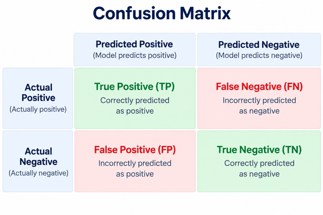
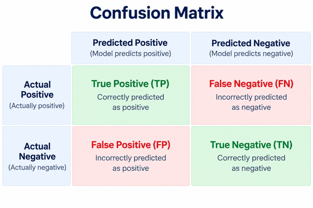
The four values above in the confusion matrix diagram are used to calculate important classification metrics such as accuracy, precision, recall, and F1 score. Let’s explore each of them in detail.

Build practical AI and software engineering skills with the Executive Post Graduate Certificate in AI-Native Software Engineering. Learn to use AI across the software development lifecycle and prepare for the evolving demands of modern engineering roles.

Understanding the Four Parts of a Confusion Matrix

Every confusion matrix machine learning for a binary classification problem is made from the four counts which are TP, TN, FP, FN. Let’s explore each of them in detail.

1. True Positive (TP)

A True Positive (TP) is a case where the model predicts the positive class and the actual outcome is also positive. 

For example, if an email is actually spam and the model also predicts it as spam, the result is a True Positive. 

2. True Negative (TN)

A True Negative is a case when the model predicts the negative class and the outcome is also negative.

For example, if a mail is not spam and the model also predicted the mail as not spam, the result is True Negative.

Also Read: Linear Regression in Machine Learning: Types, Algorithm, and Implementation

3. False Positive (FP)

A False Positive is a case where the model predicts the positive class but the result or outcome is negative. This is also called a Type I error. 

For example, if a normal mail is predicted as spam mail, this will be a False Positive.

4. False Negative (FN)

A False is a case where the model predicts the negative class but the result or outcome is positive. This is also called a Type II error.

For example, if a spam email is incorrectly classified as normal email, this will be a False negative.

The idea of a confusion matrix began during World War II. It was linked to Signal Detection Theory (SDT), developed in the 1940s. Radar operators had to identify whether a signal was an enemy aircraft or something harmless, such as birds. A False Positive meant detecting a threat that was not there, while a False Negative meant missing a real threat. This idea later became the foundation of the confusion matrix used in machine learning. 

Also Read: K Means Clustering in Machine Learning: Algorithm, Steps, Examples, and Applications

Once you know about TP, TN, FP, and FN, you can calculate several important metrics, which make up the confusion matrix formula set most commonly used to evaluate a classification model. Let’s explore those metrics.

Confusion Matrix Metrics

Common metrics are used in confusion matrix in machine learning including accuracy, precision, recall, F1 score and Specificity. Let’s explore each of them in detail.

1. Accuracy

Accuracy measures the proportion of total predictions that the model classified correctly. A higher accuracy means the model has correctly classified a larger proportion of the observations.

Confusion Matrix Formula for Accuracy:

Accuracy = (TP + TN) / (TP + TN + FP + FN)

2. Precision

Precision measures how many of the observations predicted as positive were actually positive. It is useful when False Positives are costly.

Confusion Matrix Formula for Precision:

Precision = TP / (TP + FP)

Also Read: Logistic Regression in Machine Learning: Algorithm, Types, Examples, and Applications

3. Recall

Recall measures how many of the actual positive cases were correctly identified by the model. It is especially important when missing a positive case can have serious consequences.

Confusion Matrix Formula for Recall:

Recall = TP / (TP + FN)

4. F1 Score

The F1 score combines precision and recall into a single metric. It is calculated as their harmonic mean. The F1 score is useful when you want to consider both precision and recall together.

Confusion Matrix Formula for F1 Score:

F1 Score = 2 × (Precision × Recall) / (Precision + Recall)

5. Specificity

Specificity measures how well a model identifies actual negative cases. A high specificity means the model correctly identifies a large proportion of negative cases.

Confusion Matrix Formula for Specificity:

Specificity = TN / (TN + FP)

Now let's explore how a confusion matrix is created and interpreted after a classification model makes predictions. 

Also Read: Clustering in Machine Learning: Types, Algorithms, Examples, and How It Works

How Does a Confusion Matrix in Machine Learning Work?

A confusion matrix machine learning compares each prediction made by a model with the actual answer and groups the results into four categories.

The process commonly follows these steps:

1. Train a classification model using the available dataset.

2. Use the trained model to make predictions on test data.

3. Compare the predicted labels with the actual labels.

4. Count the True Positives, True Negatives, False Positives, and False Negatives.

5. Place these values into the confusion matrix.

6. Use the values to calculate metrics such as accuracy, precision, recall, and F1 score.

For example, suppose a model predicts whether 100 customers will leave a company or not. The actual customer outcomes can be compared with the model's predictions. The resulting confusion matrix can show whether the model is correctly identifying customers who are likely to leave and customers who are likely to stay.

Also Read: Supervised vs Unsupervised Learning: Differences, Examples, and Applications

Now let's see a simple confusion matrix example to understand how its values and metrics are calculated which helps you to understand the topic more clearly.

Confusion Matrix Example

Through an actual confusion matrix example you can make the concepts far more clear than formulas alone.

Simple Binary Classification Example

Suppose a machine learning model predicts whether patients have a particular condition or not. After testing the model on 100 patients, the results are:

Here:

• TP = 40

• FN = 10

• FP = 5

• TN = 45

How to Calculate TP, TN, FP, and FN

From the matrix:

• True Positive = 40: 40 positive cases were correctly predicted.

• True Negative = 45: 45 negative cases were correctly predicted.

• False Positive = 5: 5 negative cases were incorrectly predicted as positive.

• False Negative = 10: 10 positive cases were incorrectly predicted as negative.

Now we can use these values to calculate the model's metrics by using the confusion matrix formulas we discussed above.

1. Accuracy: (TP + TN) / (TP + TN + FP + FN)

(40 + 45) / (40 + 45 + 5 + 10) = 0.85

So, the model has an accuracy of 85%.

2. Precision: TP / (TP + FP)

40 / (40 + 5) = 0.889

The precision is approximately 88.9%.

3. Recall: TP / (TP + FN)

40 / (40 + 10) = 0.80

The recall is 80%.

4. F1 Score: 2 × (Precision × Recall) / (Precision + Recall)

2 × (0.889 × 0.80) / (0.889 + 0.80) ≈ 0.842

The F1 score is approximately 84.2%.

How to Interpret the Results?

The results show that the model correctly identified most positive and negative cases. Its precision of about 88.9% means that most cases predicted as positive were actually positive.

The recall of 80% means the model identified 80% of the actual positive cases. The difference between precision and recall also shows why looking at only accuracy may not provide a complete picture of model performance.

Also Read: Support Vector Machine (SVM) in Machine Learning: Algorithm, Types, Kernels, and Examples

Now let's see how a confusion matrix in machine learning works when a model has more than two classes.

Confusion Matrix for Multiclass Classification

A confusion matrix can also be used for multiclass classification problems. Instead of two rows and two columns, it contains one row and one column for each class.

For example, a model classifying images into Cat, Dog, and Bird could have a matrix like this:

The diagonal values represent correct predictions, while the values outside the diagonal represent incorrect predictions.

For example, the value 45 means 45 actual cats were correctly classified as cats. The value 3 means three actual cats were incorrectly classified as dogs.

Now, try using the confusion matrix above to solve this exercise yourself which gives you a better understanding of how confusion matrix machine learning works.

Exercise: Analyze the Confusion Matrix

Try solving this new example yourself.

Suppose a model predicts whether emails are Spam or Not Spam. The model is tested on 200 emails, with the following results:

Using this confusion matrix, calculate:

1. True Positive (TP)

2. True Negative (TN)

3. False Positive (FP)

4. False Negative (FN)

5. Accuracy

6. Precision

7. Recall

8. F1 Score

Tip: First identify TP, TN, FP, and FN from the matrix. Then use the formulas to calculate each metric.

Once you complete the above exercise let's understand how to create a confusion matrix in Python using scikit-learn. 

Strengthen your data science skills with the Executive Post Graduate Certificate in Applied Data Science & Agentic AI. Learn to work with data, AI, and intelligent agents to build practical solutions for real-world business challenges.

How to Create a Confusion Matrix in Python

In the section you will get a complete confusion matrix python example using scikit-learn to help you implement the confusion matrix machine learning practically.

1. Calculate the Confusion Matrix Using Scikit-learn

The confusion_matrix() function from sklearn.metrics can calculate the matrix from actual and predicted labels.

from sklearn.metrics import confusion_matrix

import seaborn as sns

import matplotlib.pyplot as plt

actual = [1, 1, 1, 0, 0, 0, 1, 0]

predicted = [1, 1, 0, 0, 0, 1, 1, 0]

cm = confusion_matrix(actual, predicted)

print(cm)

Output:

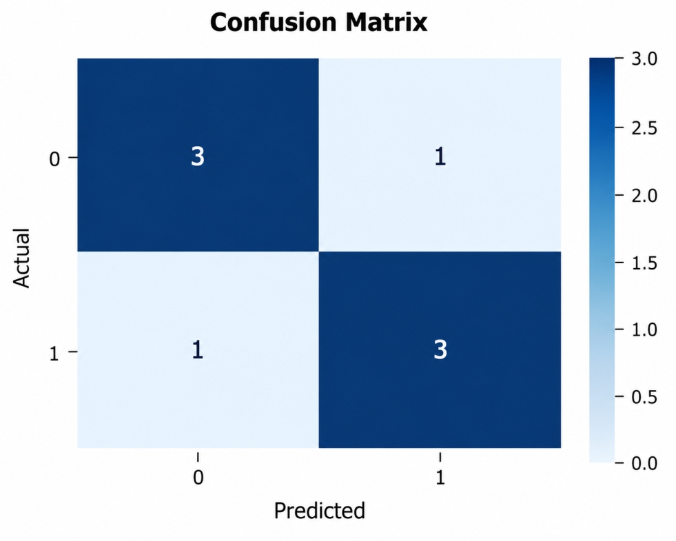
[[3 1] 

[1 3]] 

2. Visualise the Confusion Matrix as a Heatmap 

You can also visualise the confusion matrix as a heatmap:

sns.heatmap(cm, annot=True, fmt="d", cmap="Blues")

plt.xlabel("Predicted")

plt.ylabel("Actual")

plt.title("Confusion Matrix")

plt.show()

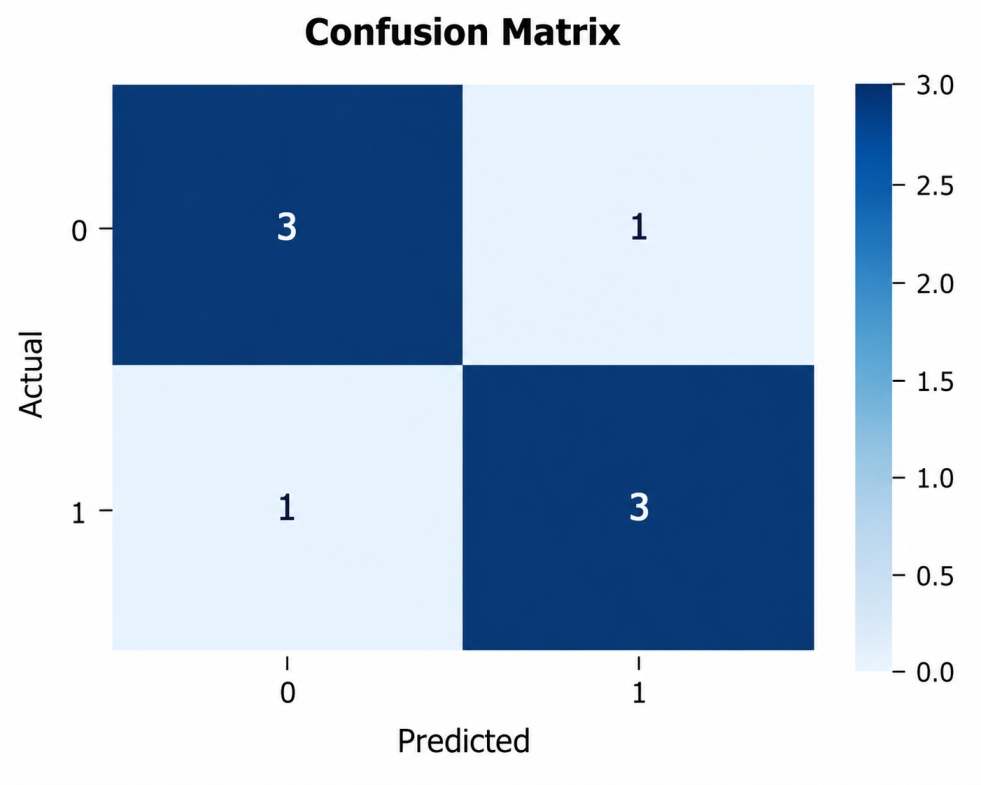
Output:

3. Calculate Classification Metrics Using Scikit-learn 

The confusion matrix can also be used with other classification metrics from scikit-learn:

from sklearn.metrics import accuracy_score, precision_score, recall_score, f1_score

print("Accuracy:", accuracy_score(actual, predicted))

print("Precision:", precision_score(actual, predicted))

print("Recall:", recall_score(actual, predicted))

print("F1 Score:", f1_score(actual, predicted))

Output:

Accuracy: 0.75

Precision: 0.75

Recall: 0.75

F1 Score: 0.75

So the model achieves 75% for all four metrics in this example. 

This approach is commonly used when evaluating classification models in Python using confusion matrix sklearn.

Also Read: K Nearest Neighbors Algorithm in Machine Learning: How It Works and Examples

Exercise: Create a Multiclass Confusion Matrix in Python

Now try the same process with a multiclass classification problem. Suppose a model classifies images into three classes: Cat (0), Dog (1), and Bird (2).

Use these values:

actual = [0, 1, 2, 0, 1, 2, 0, 2, 1, 0]

predicted = [0, 1, 2, 1, 1, 0, 0, 2, 2, 0]

Try to:

• Create the 3 × 3 confusion matrix

• Display it as a heatmap

• Calculate the overall accuracy

• Find the number of correct predictions for each class

• Identify which classes were confused with each other

Tip: For multiclass classification, the diagonal values represent correct predictions. Values outside the diagonal represent incorrect predictions.

Now let's explore what are the key advantages and limitations of using a confusion matrix for model evaluation. 

Also Read: Random Forest Algorithm in Machine Learning: Working, Types, Pseudocode

Advantages and Limitations of a Confusion Matrix

A confusion matrix is one of the most informative tools in classification evaluation, but it is also important to understand where it falls short as well.

The key advantages and limitations of Confusion matrix in machine learning are:

Advantages of a Confusion Matrix

• Provides a detailed view of correct and incorrect predictions.

• Separates False Positives from False Negatives.

• Helps calculate accuracy, precision, recall, F1 score, and specificity.

• Useful for binary and multiclass classification.

• Helps identify which classes a model is confusing.

• Can provide more information than accuracy alone.

Limitations of a Confusion Matrix

• Can become difficult to interpret when there are many classes.

• Does not directly measure model performance on regression problems.

• Individual metrics may provide an incomplete picture when considered alone.

• A confusion matrix does not explain why the model made an incorrect prediction.

• Interpretation depends on the specific application and cost of different types of errors.

Also Read: Gradient Boosting Algorithm in Machine Learning: How It Works, and Practical Examples

Conclusion

Now you have a good idea of what is confusion matrix machine learning, you have seen how it helps evaluate classification models by showing correct predictions, false positives, and false negatives. Metrics such as accuracy, precision, recall, and F1 score can then be calculated from these values.

Understanding the confusion matrix formula, examples, Python implementation, and multiclass classification can help you evaluate models more effectively and identify the types of errors they make.