Neural Network in Artificial Intelligence: Working, Types and Architecture

Quick Overview:

• A neural network is a machine learning model which is made of interconnected neurons, weights, biases, activation functions, and layers that learn patterns from data.

• Neural network architecture typically includes input, hidden, and output layers, with different architectures designed for specific tasks and types of data.

• Common types include feedforward neural networks, CNNs, RNNs, LSTMs, GANs, autoencoders, and transformers, for different types of applications.

• In this blog you will learn what is neural network in detail along with its architecture, working, types, activation functions, examples, real life application and Python Implementation.

Develop practical skills to design, build, and deploy AI products, systems, and services with the Executive Post Graduate Certificate in Building AI Products, Systems & Services. Learn to turn AI concepts into scalable, real-world solutions. 

What Is a Neural Network?

A neural network is a machine learning model which is inspired by the human brain where biological neurons process information. It uses interconnected nodes which are called neurons to identify the patterns in data to make predictions and decisions.

Your brain has billions of neurons which receive signals, process them, and pass signals to other neurons. The artificial neural networks copy this basic idea in a simpler mathematical form. 

Let’s understand this through a neural network diagram below:

An artificial neural network typically contains three types of layers:

• Input layer

• Hidden layer or layers

• Output layer

Each connection between neurons has a weight. The network also uses biases and activation functions to process information. For example, consider a neural network designed to predict whether an email is spam. The input features could include:

• Number of links

• Number of certain keywords

• Email length

• Sender information

• Frequency of specific words

Artificial Neural networks are used for tasks such as image recognition, natural language processing, speech recognition, recommendation system and predictive analytics. Neural network machine learning​ learns complex relationships between huge amounts of data and it is a core technology for many modern AI applications.

Also Read: Supervised vs Unsupervised Learning: Differences, Examples, and Applications

History of Neural Networks

The core idea behind the AI neural network​ is not new, it was developed several years ago.

• In 1943, Warren McCulloch and Walter Pitts proposed a mathematical model of an artificial neuron. 

• Later, researchers developed learning algorithms that allowed artificial neurons to adjust their behaviour based on data. 

• The perceptron, introduced by Frank Rosenblatt in 1958, became an important early neural network model. 

As computing power and access to large datasets increased, neural networks became more practical for complex tasks.

The development of backpropagation, improved hardware such as GPUs, large datasets, and modern deep learning architectures contributed to the rapid growth of neural networks in AI and today, neural networks are used in areas ranging from computer vision and speech recognition to generative AI and autonomous systems.

Also Read: Classification vs Regression in Machine Learning

Key Components of a Neural Network

Every artificial neural network is made by some combination of key components. Components used in neural network machine learning​ are:

1. Neurons (nodes): A neuron is the basic processing unit of a neural network, receiving one or more inputs, combining them, and passing the result through an activation function to produce an output.  

2. Weights: Weights are numeric values assigned to each connection between neurons, determining how much influence one neuron's output has on the neurons it connects to.

3. Biases: A bias is an additional adjustable value added to a neuron's weighted input, giving the network extra flexibility to shift its output independently of the input values alone.

4. Activation function: An activation function determines whether, and how strongly, a neuron "fires" based on its combined input, and it is what allows a neural network to model non-linear relationships rather than being limited to simple linear combinations.

5. Layers: Layers are groups of neurons that process information at the same stage of the network, organized into an input layer, one or more hidden layers, and an output layer, covered in detail in the architecture section below.

Now let’s explore the neural network architecture to understand it more better, and for understanding the neural network machine learning​ working clearly.

Neural Network Architecture

Neural network architecture refers to how neurons and layers are organized within a network. The basic AI neural network​ architecture consists of:

1. Input Layer

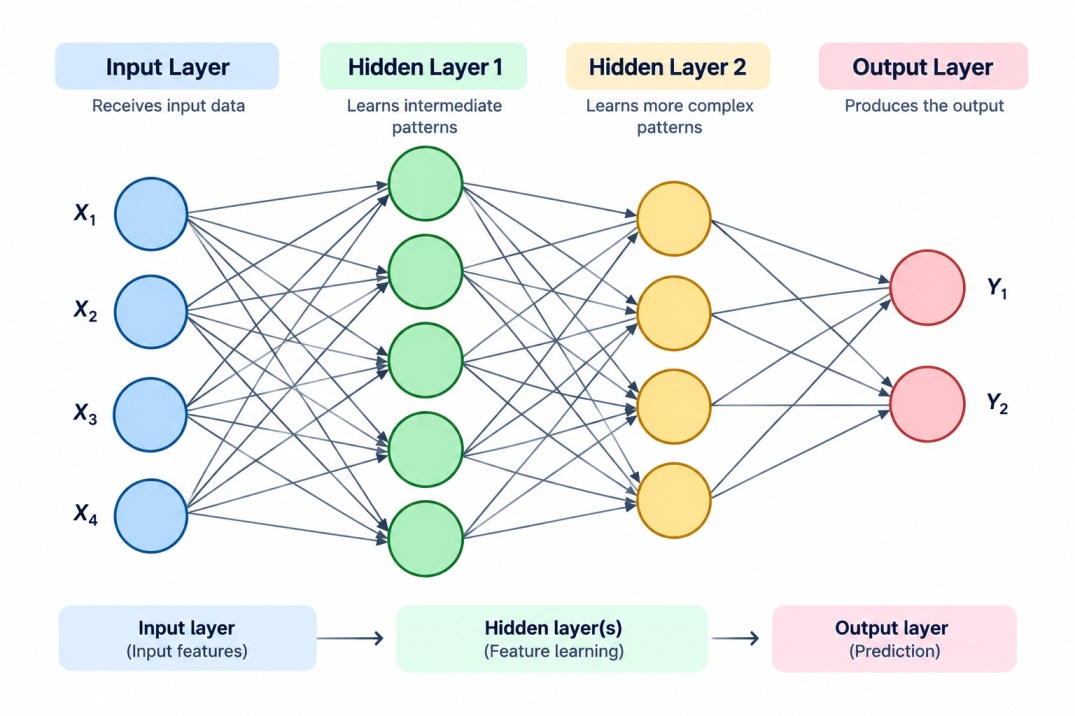
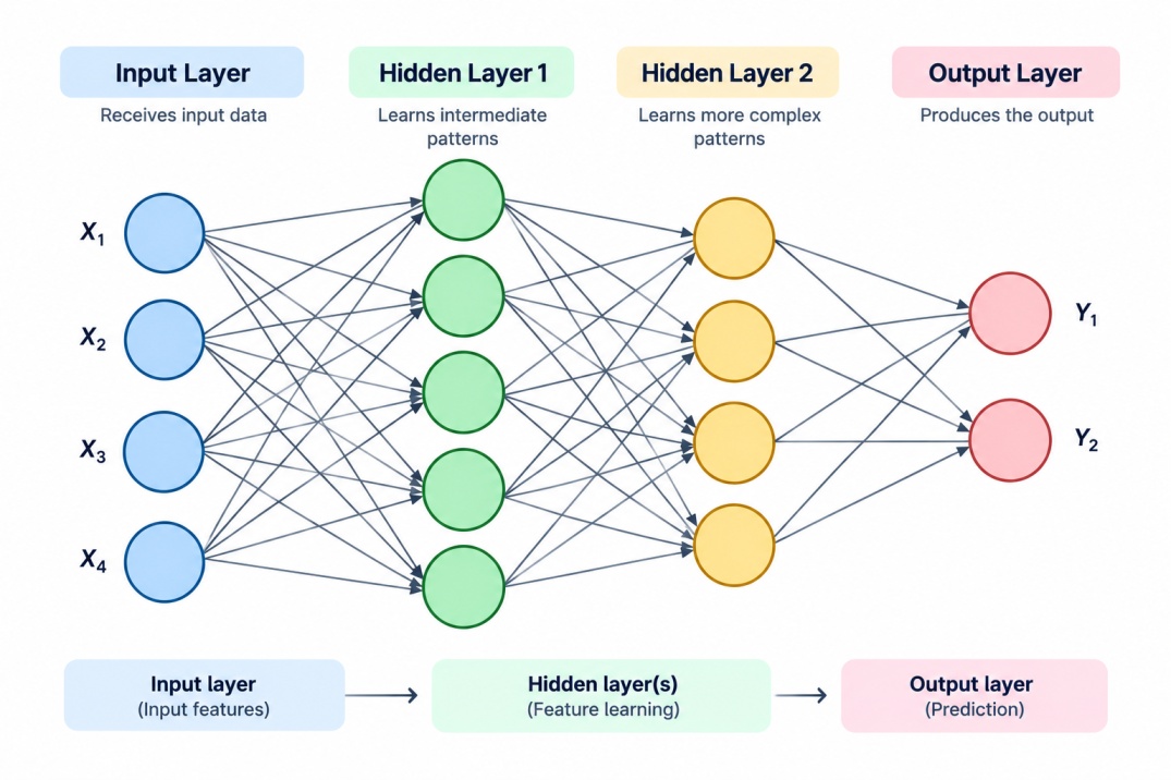
The input layer is where raw data enters the network, with one node for each feature in the dataset; it does not perform any computation itself, simply passing each feature's value into the first hidden layer.

For example, if a dataset contains five input variables, the input layer may have five input units.

2. Hidden Layers

Hidden layers perform mathematical transformations on the input data. A neural network machine learning can contain:

• One hidden layer

• Multiple hidden layers

• Hundreds of layers in some deep learning architectures

Each hidden layer learns representations from the information received from the previous layer.

The deeper the network, the more complex patterns it can potentially learn, although deeper networks also require careful training and sufficient data and computational resources.

3. Output Layer

The output layer produces the final result. Its structure depends on the task.

For example, an artificial neural network that predicts whether a customer will leave a company may have one output representing the probability of customer churn.

After exploring AI neural network​ architecture, let’s explore how the Neural Network works.

Also Read: Reinforcement Learning (RL) in Machine Learning: How It Works, Algorithms and Types

How Does a Neural Network Work?

A neural network works by processing input data through a sequence of mathematical operations. The basic process involves:

1. Input data is provided to the network.

2. Inputs are multiplied by their corresponding weights.

3. The weighted values are added together with a bias.

4. An activation function is applied.

5. The result is passed to the next layer.

6. The output layer generates the final prediction.

7. The prediction is compared with the actual target.

8. The network calculates the error.

9. Backpropagation calculates how the error relates to the model's parameters.

10. An optimization algorithm updates the weights and biases.

Now let’s explore what different types of artificial neural networks are available for different data and uses.

Also Read: Hyperparameter Tuning in Machine Learning: Methods, Techniques, and Tools

Types of Neural Networks

There are several types of neural networks, and each is designed for different types of data or tasks.

1. Feedforward Neural Network

A feedforward neural network is one of the simplest neural network architectures. Information moves in one direction:

Input → Hidden Layers → Output

There are no cycles or feedback connections. Feedforward networks can be used for tasks such as classification and regression.

2. Convolutional Neural Network

A Convolutional Neural Network, or CNN, is commonly used for image and computer vision tasks.

CNNs use convolution operations to identify local patterns such as:

• Edges

• Shapes

• Textures

• Objects

As information passes through deeper layers, the network can learn increasingly complex visual patterns.

CNNs are used in:

• Image classification

• Object detection

• Face recognition

• Medical image analysis

• Image segmentation

3. Recurrent Neural Network

A Recurrent Neural Network, or RNN, is designed to process sequential data. Unlike a basic feedforward network, an RNN can use information from previous steps when processing a sequence.

RNNs have been used for:

• Text processing

• Speech recognition

• Time-series analysis

• Language modelling

4. Long Short-Term Memory Network

Long Short-Term Memory, or LSTM, is a type of recurrent neural network. LSTMs use gates to control the flow of information through the network. This allows them to retain useful information over longer sequences.

They have been used for:

• Time-series forecasting

• Speech processing

• Text generation

• Sequence classification

5. Generative Adversarial Network

A Generative Adversarial Network, or GAN, consists of two neural networks:

• Generator

• Discriminator

The generator creates new data, while the discriminator evaluates whether the data appears real or generated. GANs have been used for image generation, data augmentation, image-to-image translation, and other generative tasks.

6. Autoencoder

An autoencoder is a neural network that learns to represent input data in a compressed form and then reconstruct it. It generally contains:

• Encoder

• Latent representation

• Decoder

Autoencoders can be used for:

• Dimensionality reduction

• Anomaly detection

• Data denoising

• Representation learning

7. Transformer Network

Transformers are neural network architectures designed to process sequences using attention mechanisms. They have become important in natural language processing and generative AI.

Transformers are used in applications such as:

• Machine translation

• Text generation

• Question answering

• Text summarisation

• Large language models

Also Read: Bias Variance Tradeoff in Machine Learning: Concept, Examples, and Techniques

Common AI Neural Network Activation Functions

Activation functions introduce non-linearity into neural networks. Without suitable non-linear activation functions, stacking multiple linear transformations would still result in a linear transformation.

Some common activation functions are:

ReLU: Short for Rectified Linear Unit, outputs the input directly if it is positive and zero otherwise; it is the most widely used activation function in modern hidden layers because it trains quickly and avoids much of the slowdown sigmoid and tanh can cause in deep networks.

Sigmoid: Breaks any input into a range between 0 and 1, historically common but now used mainly in output layers for binary classification, since it can cause training to slow down significantly in deep networks.

Tanh: Breaks input into a range between -1 and 1, offering similar behaviour to sigmoid but centred around zero, which can help training converge somewhat faster in hidden layers.

Softmax: Converts a vector of raw output values into a probability distribution across multiple classes, making it the standard choice for the output layer of a multi-class classification network.

Also Read: Clustering in Machine Learning: Types, Algorithms, Examples, and How It Works

Now let’s understand how an artificial neural network learns which makes the picture more clear.

How Do Artificial Neural Networks Learn?

Neural networks learn by adjusting their parameters based on the errors they make during training. The network compares its predictions with the actual answers and gradually changes its weights and biases to reduce the error.

The learning process generally includes the following steps:

Step 1: Initialise Parameters

The network begins with initial values for weights and biases. These values are usually set using a suitable random initialisation method. At this stage, the network has not yet learned any meaningful patterns from the data.

Step 2: Forward Pass

The training data is passed through the network layer by layer. Each neuron applies its weights, bias, and activation function to the incoming data. The final layer produces a prediction based on the patterns the network has learned so far.

Step 3: Calculate Loss

The loss function compares the model's prediction with the actual value. It produces a numerical value that represents how far the prediction is from the expected result. A higher loss generally indicates a larger prediction error.

Step 4: Calculate Gradients

During backpropagation, the network calculates gradients that show how much each weight and bias contributed to the loss. These gradients help identify which parameters need to change and in which direction.

Step 5: Update Parameters

An optimization algorithm, such as Gradient Descent or Adam, uses the calculated gradients to update the weights and biases. The goal is to make small adjustments that reduce the loss in future predictions.

Step 6: Repeat

The process is repeated across multiple batches of training data and epochs. With each cycle, the network adjusts its parameters based on the errors it observes.

As training progresses, the network gradually learns useful patterns from the training data. The aim is to reduce the loss and produce more accurate predictions on new, unseen data.

Also Read: Confusion Matrix in Machine Learning: Types, Metrics, and Examples

Neural Network Example

Simple input dataset. The XOR problem is one of the most famous small examples in neural network history, precisely because it cannot be solved by a single-layer network, which is exactly what motivated the shift toward multi-layer architectures. The dataset has just four rows: inputs of (0,0), (0,1), (1,0), and (1,1), with target outputs of 0, 1, 1, and 0, respectively, the classic exclusive-or logical pattern.

import numpy as np

np.random.seed(42)

X = np.array([[0,0],[0,1],[1,0],[1,1]])

y = np.array([[0],[1],[1],[0]])

def sigmoid(x):

    return 1 / (1 + np.exp(-x))

def sigmoid_deriv(x):

    return x * (1 - x)

# A small network: 2 inputs, 2 hidden neurons, 1 output

W1 = np.random.uniform(-1, 1, (2, 2))

b1 = np.zeros((1, 2))

W2 = np.random.uniform(-1, 1, (2, 1))

b2 = np.zeros((1, 1))

learning_rate = 0.5

for epoch in range(10000):

    # Forward pass

    hidden_output = sigmoid(np.dot(X, W1) + b1)

    final_output = sigmoid(np.dot(hidden_output, W2) + b2)

    # Backward pass

    error_output = y - final_output

    d_output = error_output * sigmoid_deriv(final_output)

    error_hidden = d_output.dot(W2.T)

    d_hidden = error_hidden * sigmoid_deriv(hidden_output)

    # Update weights and biases

    W2 += hidden_output.T.dot(d_output) * learning_rate

    b2 += np.sum(d_output, axis=0, keepdims=True) * learning_rate

    W1 += X.T.dot(d_hidden) * learning_rate

    b1 += np.sum(d_hidden, axis=0, keepdims=True) * learning_rate

print("Final predictions:")

for i in range(4):

    print(f"Input {X[i]} -> {final_output[i][0]:.4f} (rounded: {round(final_output[i][0])}), actual: {y[i][0]}")

Output:

Final predictions:

Input [0 0] -> 0.0230 (rounded: 0), actual: 0

Input [0 1] -> 0.9742 (rounded: 1), actual: 1

Input [1 0] -> 0.9742 (rounded: 1), actual: 1

Input [1 1] -> 0.0208 (rounded: 0), actual: 0

After 10,000 training passes, the mean squared error drops from 0.286 to about 0.0006. The final predictions are 0.023, 0.974, 0.974, and 0.02, which round to 0, 1, 1, and 0, correctly learning the XOR pattern. This shows why hidden layers are needed for problems that are not linearly separable.

Let’s understand through a real life example also:

Consider a simple neural network that predicts whether a student will pass an exam based on two inputs:

• Hours studied

• Attendance percentage

Suppose the dataset contains:

• The two input features are provided to the input layer.

• The hidden layer processes these values using weights, biases, and activation functions.

• The output layer produces a probability.

For example:

Input:
5 hours studied, 75% attendance

Output:
Pass probability = 0.82

If the selected decision threshold is 0.5, the model predicts:

Prediction: Pass

During training, the network compares its prediction with the actual result and adjusts its parameters to reduce future errors.

Now let’s explore how you can implement an AI neural network​ using Python.

Neural Networks in Python

Python provides several libraries for creating and training neural networks. Popular options include:

• TensorFlow

• Keras

• PyTorch

• scikit-learn

Keras can be used to build a simple neural network with relatively little code.

import numpy as np

import pandas as pd

from sklearn.model_selection import train_test_split

from sklearn.preprocessing import StandardScaler

from sklearn.neural_network import MLPClassifier

from sklearn.metrics import accuracy_score, precision_score, recall_score, f1_score

np.random.seed(42)

n = 400

income = np.round(np.random.uniform(20000, 120000, n))

credit_score = np.round(np.random.uniform(300, 850, n))

existing_loans = np.random.randint(0, 4, n)

score = (income / 120000) 0.5 + (credit_score / 850) 0.5 - existing_loans * 0.1

approved = ((score + np.random.normal(0, 0.1, n)) > 0.45).astype(int)

df = pd.DataFrame({

    "Income": income, "CreditScore": credit_score,

    "ExistingLoans": existing_loans, "Approved": approved

})

X = df[["Income", "CreditScore", "ExistingLoans"]]

y = df["Approved"]

X_train, X_test, y_train, y_test = train_test_split(

    X, y, test_size=0.2, random_state=42, stratify=y

)

scaler = StandardScaler()

X_train_scaled = scaler.fit_transform(X_train)

X_test_scaled = scaler.transform(X_test)

model = MLPClassifier(

    hidden_layer_sizes=(16, 8), activation="relu",

    solver="adam", max_iter=1000, random_state=42

)

model.fit(X_train_scaled, y_train)

y_pred = model.predict(X_test_scaled)

print("Accuracy:", accuracy_score(y_test, y_pred))

print("Precision:", precision_score(y_test, y_pred))

print("Recall:", recall_score(y_test, y_pred))

print("F1-score:", f1_score(y_test, y_pred))

print("Number of layers:", model.n_layers_)

Output:

Accuracy: 0.8375

Precision: 0.8666666666666667

Recall: 0.8478260869565217

F1-score: 0.8571428571428571

Here, hidden_layer_sizes=(16, 8) builds a network with two hidden layers of 16 and 8 neurons, activation="relu" uses the ReLU function covered earlier for the hidden layers, and solver="adam" selects a widely used variant of gradient descent. Running this on the sample dataset produces an accuracy of 0.8375, a precision of 0.8667, a recall of 0.8478, and an F1-score of 0.8571, with model.n_layers_ confirming 4 total layers: the input layer, the two hidden layers, and the output layer.

At this point the neural network machine learning​ is clear for you with a practical implementation also. Now let’s see where it is used in real life applications.

Real-World Applications of Neural Networks

Neural networks power a wide range of applications already present in everyday technology, and AI neural network systems now sit behind tools that hundreds of millions of people use daily. 

Some common applications include:

Every technology comes with some pros and cons, so now let’s explore some of the advantages and disadvantages of a neutral network.

Advantages and Limitations of Neural Networks

Neural networks can solve complex problems, but they also have limitations that need to be considered.

Advantages of Neural Networks

• Can Learn Complex Patterns: It can learn non-linear relationships that may be difficult to capture using simpler models.

• Suitable for Large and Complex Data: They can process different types of data, including numerical data, images, audio, and text.

• Useful for Automated Feature Learning: Deep neural networks can learn representations from raw or minimally processed data in many applications.

• Can Support High-Performance Applications: With appropriate data, architecture, training, and computational resources, neural networks can perform effectively on many complex tasks.

• Flexible Architecture: Different architectures can be designed for different problems. CNNs are commonly used for image-related tasks, while recurrent architectures and transformers can handle sequential or language-related tasks.

Limitations

• Requires Large Amounts of Data for Some Tasks: Complex networks may require substantial training data to learn effectively.

• Computationally Expensive: Training large networks can require significant computing power and memory.

• Can Be Difficult to Interpret: Neural networks can contain many parameters and complex transformations, making their decisions harder to explain than those of some simpler models.

• Training Can Take Time: Large models can require considerable time to train, especially when working with large datasets.

Conclusion

So, what is neural network? A neural network is a machine learning model made up of interconnected neurons that learn patterns from data. It processes information through input, hidden, and output layers and adjusts its weights and biases during training.

Different network architectures are suited to different problems. CNNs are widely used for computer vision, RNNs and LSTMs can process sequential information, autoencoders can learn compressed representations, GANs can generate data, and transformers are widely used in modern NLP and generative AI.