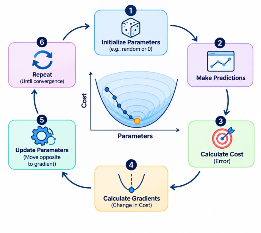
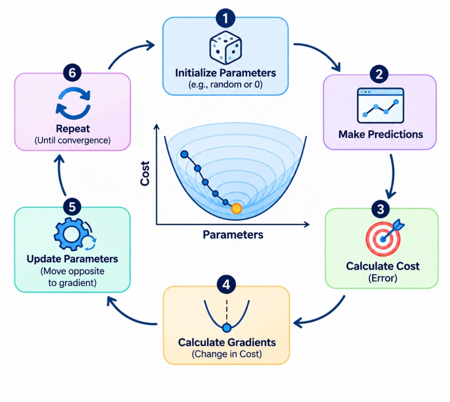
Initial parameter values are chosen, often a randomly selected small number or 0.
Predictions are made given the current parameters.
Calculate cost (error between predicted and correct values).
Calculate gradients. This will show the change in cost for changing each parameter.
Update parameters: move each parameter in the opposite direction of the gradient, by a small amount.
Repeat until cost is no longer decreasing, or after a fixed number of iterations.
Each time we go through a batch of training data we call that an epoch. Usually many epochs of training are required. The learning curve can be plotted (epochs vs cost), to see if the algorithm is converging.
Working Example
Suppose the cost function is f(x) = x squared, whose lowest point is at x = 0. The gradient is 2x.
Start at x = 5 with a learning rate of 0.1. Each update subtracts 0.1 times the gradient, so x becomes 4, then 3.2, then 2.56, then 2.05, and keeps shrinking toward zero.
Each step is smaller than the last because the slope flattens as the algorithm approaches the minimum.
Types of Gradient Descent
The main types of gradient descent differ in one choice: how much training data is used to compute each gradient before updating the parameters. That choice changes speed, stability, and memory use.
Factor | Batch Gradient Descent | Stochastic Gradient Descent | Mini-Batch Gradient Descent |
Data per update | The entire training set | One example | A small group, such as 32 to 256 examples |
Updates per epoch | One | As many as there are examples | Dataset size divided by batch size |
Speed per update | Slow on large datasets | Very fast | Fast |
Path to minimum | Smooth and stable | Noisy and jumpy | Moderately smooth |
Memory use | High, needs all data | Low | Moderate |
Hardware efficiency | Good for vectorized math | Poor, little parallel work | Very good on GPUs |
Can escape shallow local minima | Less likely | More likely because of noise | Somewhat likely |
Typical use | Small datasets and convex problems | Online learning and very large data | Default for deep learning |
Batch Gradient Descent
Batch gradient descent computes the gradient using every training example before making a single update. This gives a smooth, stable path toward the minimum and exact gradients. The drawback is cost. On a dataset with millions of rows, one update means one full pass over the data, which is slow and memory heavy. It works well for small datasets and convex problems.
Stochastic Gradient Descent
Stochastic gradient descent, often called SGD, updates the parameters after each single training example. Updates are cheap and frequent, so progress starts quickly and the method can handle huge or streaming datasets.
The gradient from one example is a noisy estimate, so the cost jumps around instead of falling smoothly. This noise can actually help the algorithm leave shallow local minima, but it also means the final answer may keep wobbling around the minimum unless the learning rate is reduced over time.
Mini-Batch Gradient Descent
Mini-batch gradient descent splits the data into small groups and updates after each group. It keeps much of the stability of batch updates and most of the speed of stochastic updates, and it takes full advantage of GPU parallelism. For these reasons, mini-batch is the standard choice in deep learning, and when people say SGD in a deep learning library they usually mean mini-batch SGD.
How to Implement Gradient Descent in Python?
The best way to understand the gradient descent algorithm is to write it.
The example below fits a straight line to noisy data using NumPy only. It implements all three types of gradient descent, batch, stochastic, and mini-batch, so you can compare them on the same problem. The data follows the rule y = 4 + 3x plus random noise, so a good model should learn an intercept near 4 and a slope near 3.
import numpy as np
rng = np.random.default_rng(42)
# Synthetic data: y = 4 + 3x + noise
n = 200
x = rng.uniform(0, 2, n)
y = 4 + 3 * x + rng.normal(0, 0.5, n)
X = np.c_[np.ones(n), x] # add a bias column
def mse(theta):
return np.mean((X @ theta - y) ** 2)
def gradient(theta, Xb, yb):
# Gradient of mean squared error: (2/m) * X^T (X.theta - y)
return (2 / len(yb)) * Xb.T @ (Xb @ theta - yb)
def batch_gd(lr=0.1, epochs=200):
theta = np.zeros(2)
for _ in range(epochs):
theta -= lr * gradient(theta, X, y)
return theta
def stochastic_gd(lr=0.02, epochs=50):
theta = np.zeros(2)
for _ in range(epochs):
for i in rng.permutation(n):
theta -= lr * gradient(theta, X[i:i+1], y[i:i+1])
return theta
def minibatch_gd(lr=0.05, epochs=100, batch_size=32):
theta = np.zeros(2)
for _ in range(epochs):
idx = rng.permutation(n)
for start in range(0, n, batch_size):
b = idx[start:start + batch_size]
theta -= lr * gradient(theta, X[b], y[b])
return theta
for name, fn in [("Batch", batch_gd), ("Stochastic", stochastic_gd), ("Mini-batch", minibatch_gd)]:
theta = fn()
print(f"{name:11s} intercept={theta[0]:.2f} slope={theta[1]:.2f} MSE={mse(theta):.3f}")
Running it prints:
Batch intercept=3.84 slope=3.17 MSE=0.249
Stochastic intercept=3.76 slope=3.11 MSE=0.269
Mini-batch intercept=3.84 slope=3.15 MSE=0.249
All three methods land close to the true values of 4 and 3. The small gap comes from the random noise in the data, which no method can remove.
The batch and mini-batch versions reach almost the same error, while stochastic gradient descent finishes with a slightly higher error because its updates are noisier. The only difference between the three functions is how many rows feed each call to the gradient function, which is exactly the difference described in the types section.
Hands-On Exercise: Implement Gradient Descent in Python
Now that you have implemented batch, stochastic, and mini-batch gradient descent, try building a simple gradient descent algorithm yourself.
Problem Statement:
You are given a dataset containing input values (x) and their corresponding output values (y). Your task is to train a simple linear regression model using gradient descent.
Step 1: Create the dataset
Start with the following Python code:
import numpy as np
x = np.array([1, 2, 3, 4, 5])
y = np.array([3, 5, 7, 9, 11])
w = 0.0
b = 0.0
learning_rate = 0.01
epochs = 100
Step 2: Complete the coding exercise
Fill in the missing sections to train the model.
for epoch in range(epochs):
# Calculate predictions
y_pred = __________
# Calculate the error
error = __________
# Calculate gradients
dw = __________
db = __________
# Update weight and bias
w = __________
b = __________
if epoch % 20 == 0:
print("Epoch:", epoch, "MSE:", error)
print("Final weight:", w)
print("Final bias:", b)
Step 3: Experiment with different learning rates
Run your code with these learning rates:
Observe how the model's error changes with each learning rate.
What You Should Learn?
After completing this exercise, you will understand:
How to implement gradient descent using Python.
How weights and biases change during model training.
How learning rates affect training speed.
How repeated updates help a model learn from its errors.
Challenge: Modify the code to train the model for 500 epochs. Can you get the final weight close to 2 and the bias close to 1?
Advantages and Disadvantages of Gradient Descent
Every machine learning algorithm and method comes with its own advantages and disadvantages, so now let’s explore them for gradient descent below:
Advantages | Disadvantages |
Easy to understand and compute | Very sensitive to learning rate |
Can be used with nearly any differentiable loss function | Can get stuck in local minima and saddle points in non-convex problems |
Can scale well to very large datasets and large numbers of parameters | Does not converge quickly on poorly scaled/ill conditioned data |
Mini-batch/stochastic methods are memory efficient | Batch gradient descent is slow and computationally expensive on large datasets |
Available in all major machine learning libraries | Stochastic gradients can be very noisy, may not converge exactly |
Several improvements (like Adam) make it fast and stable | Only works on differentiable functions. Not directly suited to discrete problems |
Basis of training for deep learning and large language models | Vanishing or exploding gradients in very deep networks |
Conclusion
Understanding the concept of gradient descent, the different methods and implementation in python will provide learners with a good understanding of how models are trained.
In order to fully understand how gradient descent works, it is best to experiment with different learning rates and data sets. This allows learners to relate the theory behind gradient descent with training real models.